Equal-Area Map Projections with Basemap and matplotlib/pylab

PDF [1] (read as slides)

Org [2] (reproduce)

Plotting global equal area maps with python, matplotlib/pylab and Basemap.

1 Problem

1.1 lat/lon pixels misrepresent areas

Projected B_columns
1. Simple Flat BMCOL B_block
2. Globe BMCOL
Note B_ignoreheading

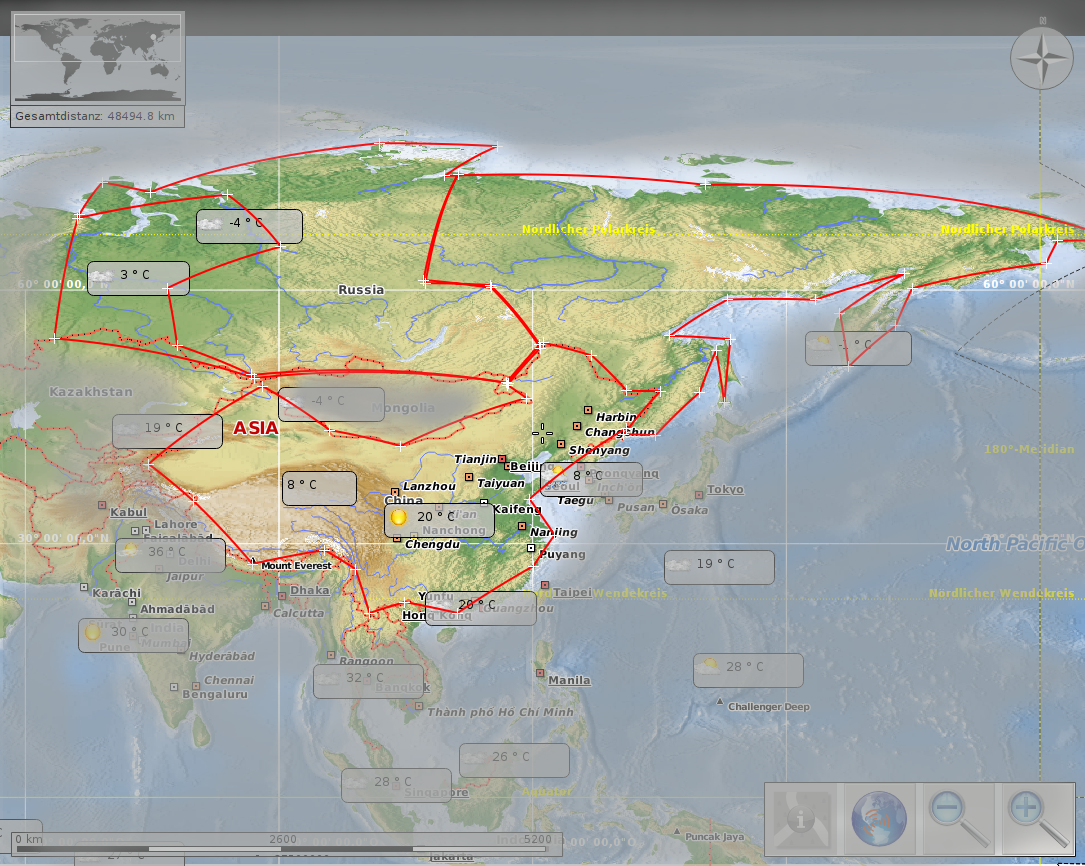
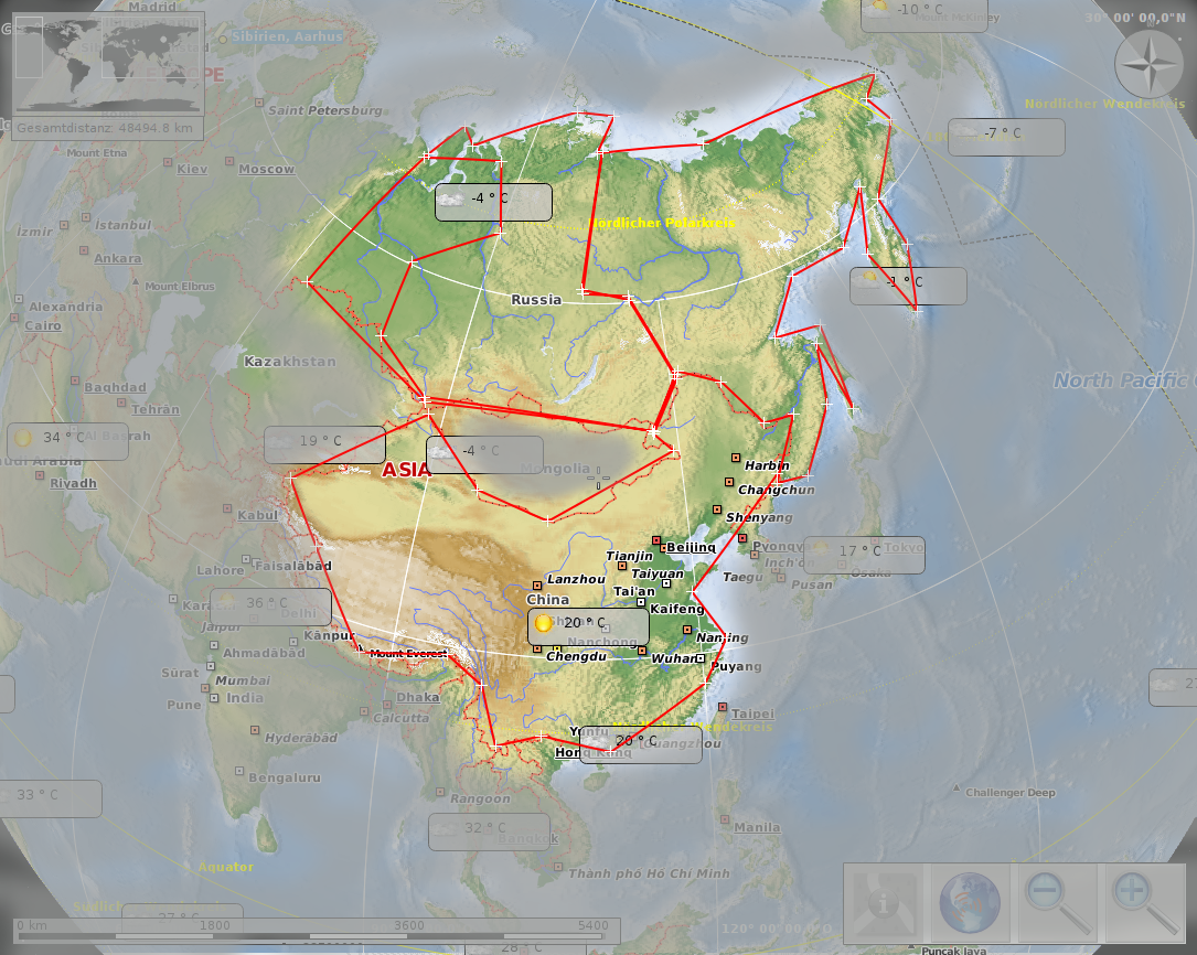
Sibiria 13,1 · 10⁶ km² vs. china 9.7 · 10⁶ km²

Maps thanks to Marble Desktop Globe [3] and Open Street Map [4], available under CC by-sa [5] and Open Data Commons Open Database License (ODbL) [6].

2 Map-Notes

2.1 Map Projections

Maps B_columns
1. Hobo-Dyer BMCOL B_block
  - Rectangle
  - equidistant longitude
  - longitude/latitude over the Mediterranean Sea (more exactly: \(37.5^\circ\))
  - Similar Maps: Gall-Peters (thinner), Lambert (wider)
  - Basemap: equal area cylindrical (cea) with lat_ts=37.5
2. Hammer BMCOL B_block
  - Elliptic
  - Low distortion at the poles
  - 2:1 → 2 per page
  - the earth appears round without making it hard to recognize patterns
  - Similar Maps: Mollweide (more distorted at the poles, parallel latitudes)
  - Basemap: hammer
3. Flat Polar Quartic B_block BMCOL
  - Elliptic with polar cuts
  - parallel latitudes
  - Standard parallels at \(33^\circ 45' N/S\)
  - poles are \(\frac{1}{3}\) the equator
  - Similar: Eckart IV (poles are half the equator)
  - Basemap: mbtfpq

3 Plotted

3.1 Hobo-Dyer

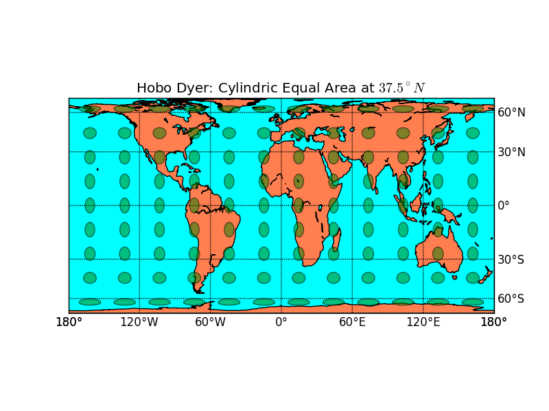
m = map.Basemap(projection='cea', lat_ts=37.5)
outfile = "hobo-dyer.png"
pl.title("Hobo Dyer: Cylindric Equal Area at $37.5^\\circ N$")

3.2 Hammer

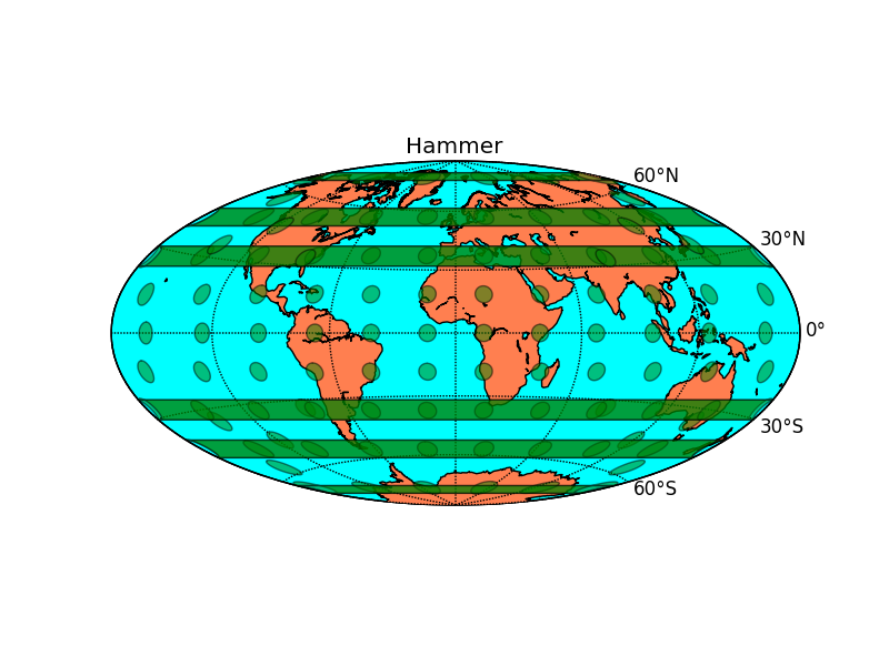
m = map.Basemap(projection='hammer', lon_0=0)
outfile = "hammer.png"
pl.title("Hammer") # latex-test: $\frac{1}{2}$

3.3 Flat Polar Quartic

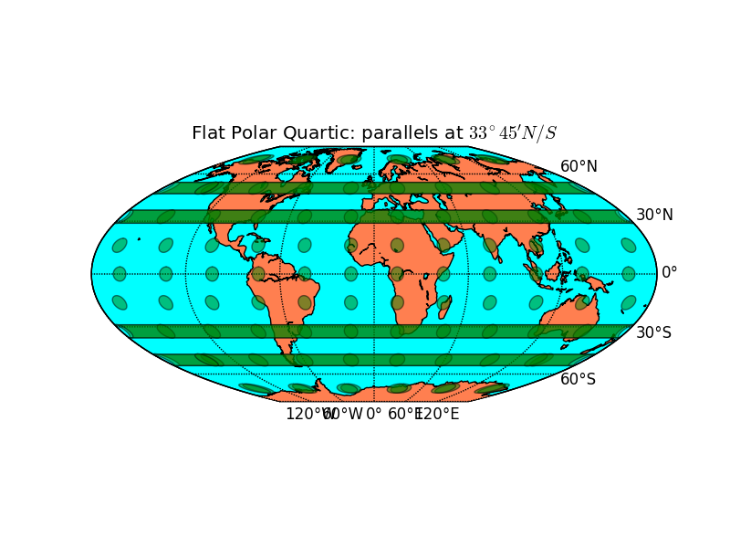
m = map.Basemap(projection='mbtfpq', lon_0=0)
outfile = "flatpolarquartic.png"
pl.title("Flat Polar Quartic: parallels at $33^\\circ 45' N/S$")

4 Other maps

4.1 Other Equal Area map types

Goode homolosine: Split, focus on land or ocean, straight latitude parallels, approximately preserve most shapes. Not available in matplotlib.
Eckert IV: Like Flat Polar Quartic, parallels at 40° 30' N/S, poles are half the equator.
Lambert cylindrical equal area: Like Hobo Dyer, very wide, shapes at the equator are correct.
Gall Peters: Like Hobo Dyer, appears more distorted than Hobo-Dyer, shapes over europe correct (45°).
Mollweide: Like Hammer with straight latitude parallels.
Werner: It’s a heart :) - focus on a hemisphere without ignoring the rest. General case: Bonne.
Tobler: General case leading to Lambert, Mollweide, Mollington and a few more — also see Tobler1973 [7] after you manage to gnawl through the paywall…
Collignon: Triangle, for cosmic microwave background.

5 Conclusing

5.1 Maps I plan to use

Maps B_columns
1. Hobo-Dyer BMCOL B_block
  
  To show regional fluxes and longitudinally constrained regions: Easy to spot on rectangular grid.
2. Hammer B_block BMCOL
  
  To show a global overview: Helps the understanding of global data because it appears most similar to a real earth while including the whole earth surface.
3. Flat Polar Quartic B_block BMCOL
  
  For mainly latitudinally constrained regions: Straight latitudinal lines and high latitudinal resolution near the poles.

6 Thank you!

6.1 Thank you for listening!

Questions? B_block BMCOL

7 Appendix: Supporting functions

7.1 Basemap Imports

Basic imports for plotting with Basemap.

# basemap, pylab and numpy for plotting
import mpl_toolkits.basemap as map
import pylab as pl
import numpy as np
# netcdf for reading the emission files
import netCDF4 as nc

Basemap: http://matplotlib.org/basemap/ [8]
Pylab: http://www.scipy.org/PyLab [9]
Numpy: http://www.numpy.org/ [10]
NetCDF: http://code.google.com/p/netcdf4-python/ [11]

7.2 Draw a map

Commands to draw a map. If no emission data is available, use the default fill color for continents. Requires previous imports and a basemap setup as done in the plot snippets for the individual maps.

<<addmapfeatures>>
<<addindicatrix>>
try:
  <<addemissions>>
  <<addcolorbar>>
except RuntimeError: # recover from missing fluxfile
  m.fillcontinents(color='coral',lake_color='aqua')
pl.savefig(outfile)
return "./" + outfile + ""

7.3 Map features

Commands to add visual orientation to a map.

# add map lines
m.drawcoastlines()
# only fill continents if we do not plot emissions
# m.fillcontinents(color='coral',lake_color='aqua')
m.drawparallels(np.arange(-90.,120.,30.), 
                labels=[False,True,True,False])
m.drawmeridians(np.arange(0.,420.,60.), 
                labels=[True,False,False,True])
m.drawmapboundary(fill_color='aqua')

7.4 Tissots Indicatrix

Add Tissots Indicatrix to visualize distortion.

# draw tissot's indicatrix to show distortion.
for y in np.linspace(m.ymax/20,19*m.ymax/20,9):
    for x in np.linspace(m.xmax/20,19*m.xmax/20,12):
        lon, lat = m(x,y,inverse=True)
        poly = m.tissot(lon,lat,4.0,100,
                        facecolor='green',
                        zorder=10,alpha=0.5)

7.5 Plot emissions

Plot Carbontracker emissions on a basemap (m).

# d = nc.Dataset("/run/media/arne/3TiB/CTDAS-2013-03-07-2years-base-data/"
#                "analysis/data_flux1x1_weekly/flux_1x1.nc")
d = nc.Dataset("UNPUBLISHED")
biocovmean = np.mean(
    d.variables["bio_flux_prior_cov"][:,:,:], axis=0)
# projection: matplotlib.org/basemap/users/examples.html
lons, lats = pl.meshgrid(range(-180, 180), 
                         range(-90, 90))
x, y = m(lons, lats)
# choose my standard color range: vmin = -0.5*vmax
vmax = max(abs(np.max(biocovmean)), 
           2 * abs(np.min(biocovmean)))
vmin = -0.5*vmax
m.pcolor(x, y, biocovmean, shading='flat', 
         vmin=vmin, vmax=vmax) # pcolormesh is faster

7.6 Nice colorbar

Add a nice colorbar to the plot.

pl.rcParams.update({"text.usetex": True, 
                    "text.latex.unicode": True})
colorbar = pl.colorbar(orientation="horizontal", 
                       format="%.2g") # scientific
colorbar.set_label("$CO_{2}$ fluxes [$\\frac{mol}{m^2 s}$]")

Author: Arne Babenhauserheide

Emacs [12] 24.3.1 (Org [13] mode 8.0.2)

Validate XHTML 1.0 [14]

Anhang	Größe
flatpolarquartic.png [15]	127.57 KB
hobo-dyer.png [16]	139.26 KB
hammer.png [17]	138.15 KB
sibiria-china-flat.png [18]	1.14 MB
sibiria-china-globe.png [19]	1.14 MB
equal-area-map-projections.pdf [1]	3.06 MB
equal-area-map-projections.org [2]	10.19 KB