For or about scientific work.
science [1] in a dent:
(1) Form a theory. (2) design an experiment to test the theory. (3) do it. (4) Adjust the theory, if needed → (2)
→ written in GNU social [2].
Please feel free to use it!
If that’s to brief:
→ the scientific method, explained very basically and simply [3].
and
That’s not faith. It’s theory. The difference is that there’s a clearly defined way to adjust the theory, when it’s wrong.
German version: Die Wissenschaftliche Methode in 130 Zeichen [4]
Naturally this is still vastly oversimplified, but that’s the price you pay by trying to explain a complex system in 140 characters. What’s to remember: theory and experiment go side by side and fertilize each other. New theories allow finding new experiments which answer questions in the theories and allow finding new theories (or changes to old theories – or tell us which direction of fleshing out theories will likely be useful).
PS: If you have other dents or tweets about science, please feel free to add and link them in a comment [5].
Just like this text they need to be licensed under free licenses [6].
If this should prove to be right, it’s serious.
I’m not an expert on all the topics brought together in the paper, but I never saw stronger scientific writing than what I now read in the peer-reviewed publication, and the topics I do know are represented correctly.
Update 2018-09-03 by Aengenheyster et al. 2018 [7]: For »reaching the 1.5 K target […] MM would be required to start in 2018 for a probability of 67%.« MM means getting a 2% increase of the share of renewables every year. This is still a 33% risk of failure!
Update: Hansen 2017: Young people's burden: requirement of negative CO₂ emissions [8] — a last, desperate chance to prevent what is shown in the paper linked below.
Even if you don’t think you get new information from the paper, if you have an interest in scientific writing, I strongly suggest reading the paper:
It is long. And great. And Open Access.
If you don’t want to read that much, you can watch James Hansen explain the gist himself:
https://www.youtube.com/watch?v=JP-cRqCQRc8
@Article{Hansen2016,
AUTHOR = {Hansen, J. and Sato, M. and Hearty, P. and Ruedy, R. and Kelley, M. and Masson-Delmotte, V. and Russell, G. and Tselioudis, G. and Cao, J. and Rignot, E. and Velicogna, I. and Tormey, B. and Donovan, B. and Kandiano, E. and von Schuckmann, K. and Kharecha, P. and Legrande, A. N. and Bauer, M. and Lo, K.-W.},
TITLE = {Ice melt, sea level rise and superstorms: evidence from paleoclimate data,
climate modeling, and modern observations that 2 °C global warming
could be dangerous},
JOURNAL = {Atmospheric Chemistry and Physics},
VOLUME = {16},
YEAR = {2016},
NUMBER = {6},
PAGES = {3761--3812},
URL = {http://www.atmos-chem-phys.net/16/3761/2016/},
DOI = {10.5194/acp-16-3761-2016},
ABSTRACT = {
We use numerical climate simulations, paleoclimate data, and
modern observations to study the effect of growing ice melt from
Antarctica and Greenland. Meltwater tends to stabilize the ocean
column, inducing amplifying feedbacks that increase subsurface
ocean warming and ice shelf melting. Cold meltwater and induced
dynamical effects cause ocean surface cooling in the Southern
Ocean and North Atlantic, thus increasing Earth's energy
imbalance and heat flux into most of the global ocean's
surface. Southern Ocean surface cooling, while lower latitudes
are warming, increases precipitation on the Southern Ocean,
increasing ocean stratification, slowing deepwater formation, and
increasing ice sheet mass loss. These feedbacks make ice sheets
in contact with the ocean vulnerable to accelerating
disintegration. We hypothesize that ice mass loss from the most
vulnerable ice, sufficient to raise sea level several meters, is
better approximated as exponential than by a more linear
response. Doubling times of 10, 20 or 40 years yield multi-meter
sea level rise in about 50, 100 or 200 years. Recent ice melt
doubling times are near the lower end of the 10–40-year range,
but the record is too short to confirm the nature of the
response. The feedbacks, including subsurface ocean warming, help
explain paleoclimate data and point to a dominant Southern Ocean
role in controlling atmospheric CO2, which in turn exercised
tight control on global temperature and sea level. The
millennial (500–2000-year) timescale of deep-ocean ventilation
affects the timescale for natural CO2 change and thus the
timescale for paleo-global climate, ice sheet, and sea level
changes, but this paleo-millennial timescale should not be
misinterpreted as the timescale for ice sheet response to a
rapid, large, human-made climate forcing. These climate feedbacks
aid interpretation of events late in the prior interglacial, when
sea level rose to +6–9 m with evidence of extreme storms while
Earth was less than 1 °C warmer than today. Ice melt cooling of
the North Atlantic and Southern oceans increases atmospheric
temperature gradients, eddy kinetic energy and baroclinicity,
thus driving more powerful storms. The modeling, paleoclimate
evidence, and ongoing observations together imply that 2 °C
global warming above the preindustrial level could be
dangerous. Continued high fossil fuel emissions this century are
predicted to yield (1) cooling of the Southern Ocean, especially
in the Western Hemisphere; (2) slowing of the Southern Ocean
overturning circulation, warming of the ice shelves, and growing
ice sheet mass loss; (3) slowdown and eventual shutdown of the
Atlantic overturning circulation with cooling of the North
Atlantic region; (4) increasingly powerful storms; and (5)
nonlinearly growing sea level rise, reaching several meters over
a timescale of 50–150 years. These predictions, especially the
cooling in the Southern Ocean and North Atlantic with markedly
reduced warming or even cooling in Europe, differ fundamentally
from existing climate change assessments. We discuss observations
and modeling studies needed to refute or clarify these
assertions.},
}
Report: Arctic Is Unraveling [13], discusses assessment Snow, Water, Ice and Permafrost [14], notes the article rising tide [15] — sounds more like Hansen was right [9].
Again [16] (see “20 years later” [17], from 2008).
James Hansen, 2016, “Ice melt, sea level rise and superstorms”…
…and what I can say clearly [18] (with a video where he explains the results).
To share this briefly:
Report: Arctic Unraveling, discusses assessment, notes rising tide — sounds more like Hansen was right. links: http://draketo.de/node/764 [19]
On 2015-08-27, Researchers from the Reproducibility Project: Psychology [20] reported that in 100 reproduction studies, only “47% of original effect sizes were in the 95% confidence interval of the replication effect size” (RPP SCIENCE 2015 [21], an overview of the results is available in Scientific American [22]; in german from DLF Forschung Aktuell [23]).
I take this worrying result as cue to describe current challenges to scientific publishing and measures to address them — including reproduction experiments, and what to do if they contest previously published and referenced work.
Scientific publishing has come a long way since its beginning, and its principles have allowed it to scale up from a few hundred active scientists worldwide to conferences with tens of thousands of people for a given topic. But in the last few years it hit its limits. It becomes harder each year to keep up with the amount of new papers being published and even scientists from similar fields repeatedly reinvent the same methods. To scale further and to continue to connect the scientific community, it must adapt to make it easier to get an understanding of the current state of science and keep up to date with new findings.
To grow from these challenges, scientific publishing needs to
Before I start with my critique of scientific publishing, I want to show where it really shines. This will put its shortcomings in the proper perspective and also serve as a reminder about methods proven by time. In this part I will focus on the aspects of scientific publishing which help dealing with a huge amount of information.
I will also contrast these aspects to ordinary websites, because these have become the standard information medium for non-scientists, yet they took up technology much faster than scientific publishing, which allowed some non-scientific publications to get on par with scientific publications in many aspects and even surpass them in a few.
Scientific publications are expected to have a title, keywords, an abstract, an introduction and conclusions - in addition to any other content they have. This makes it easy for readers to choose how deep they want to delve into the topic of the paper.
All this taken together creates a medium where every reader can decide how much information he or she wants to ingest. This allows priorizing a specific field while still getting a rough understanding of the larger developments happening in similar topics.
Where websites typically only provide one or two representations of any given topic - often title plus teaser and the main text - scientific publications provide several layers of information which are all useful on their own.
While the internet allowed ordinary publications to catch up a lot via hyperlinks (though these are still mostly used by hobby-writers and not so much by big newspapers), scientific publication still holds the gold standard for referencing other works in a robust way.
They include the title, the author, the journal, the date of publication and a link. Even if the journal dies and the DOI system breaks, a paper can still be found in third party databases like university libraries.
In the internet however, links regularly break, even those referenced in court cases. So here the web still has a lot to learn from the tried and true practices of scientific publishing.
(in the meantime, if you’re a blogger yourself, please preserve your links [26] (german original [27]))
The different levels of information and the robust references create a system which managed to sustain its quality during a growth in the number of researchers and publications by several orders of magnitude.
These two topics aren’t the only strengths of scientific publishing (which for example also include the peer review process in which a trusted editor asks people from the same field to provide high-quality feedback), but they are the most important strengths for the topics in which the next part identifies challenges that need to be resolved to preserve the integrity of scientific publications and to avoid and reduce the fragmentation of science by keeping researchers connected with current work from other groups.
The gist of the challenge of scientific publishing can be summarized in two questions:
Journals are already trying to tackle both of these, but the current steps fall far short of solving the problem.
Suddenly you realize that there is a group of scientists in Korea who also work in your field.
This actually happened: I shared a paper with experts in the field who did not even know that the group doing the research existed.
The problem behind this experience is that the number of scientists increased more than a hundred fold (at EGU more than 15000 people met, and that’s only for earth sciences), but scientific publishing still works similar to how it worked when there were only a few hundred (communicating) scientists worldwide. And the pressure to publish as much as possible intensifies the problem a lot.
In a field like Physics of the Atmosphere, hundreds of papers are published every month. Even the reading list filtered by interest which I get per E-Mail every week contains several tens of papers per journal. And when I started to dive into my research field at the beginning of my PhD, a huge challenge was to get the basic information. It’s easy to find very detailed information, but getting the current state of scientific knowledge for a given field takes a lot of effort, especially if you don’t start in a group working on the same topic. So how should scientists keep a general knowledge of the broader field, if it’s already hard to get into one given field?
The current answers are review papers and books. Good review papers allow understanding a core topic of a given scientific community within a few days. A nice example is Data assimilation: making sense of Earth Observation [28]. A book gives a good overview of a given field, but it requires a hefty time investment. So how do you keep a general understanding of other fields? How can we avoid reinventing the wheel again and again, just in different contexts?
A simple idea to achieve this would be to create a hierarchy of quarterly overviews:
With every overview including two aspects:
The core changes would be suggested reading for all scientists in the given field, while the state of scientific knowledge would allow people to get up to speed in a given field, or to understand something interesting, and provide a path to the more detailed reviews and papers.
Assuming that on average 2-3 broad fields and subgroups are interesting to a scientist, this would allow keeping up to date with scientific development by reading one overview paper per month, and it would allow getting a broad understanding of many fields by reading the overview of an additional field every quarter.
These structured overviews would reconnect science.
To support the creation of the overviews, we might need more dedicated, paid overview writers.
Part of this job is currently done by publications like Annual Reviews [29], Physik-Journal [30] (german) and Scientific American [31] (in order of decreasing specialization), and awareness of the need to reconnect science could make it possible to extend these and similar to make it easier to acquire and keep a good understanding of the current state of science.
The second big question is: “How do you know that you can trust this paper?” To be able to trust the results shown in any paper, there are two aspects:
The first problem can be tackled by requiring scientists to share the data and programs they analyzed, so others can reproduce the results (plots, table content and so on) with as little effort as possible. Ideally the paper should use something like autotools [32] and org mode [33] (german original [34]) to create a distribution package which allows others to reproduce the paper straight from the data and ensures that the data in the package actually suffices to generate the results. This would ensure that papers provide all the small details which might not seem worthy of publication on their own but can be essential to reproduce the results with a new experimental setup.
The article Sloppy Papers [35] (by Dennis Ogbe, 2016-04-05) provides an example of the pain caused by non-reproducible publishing; for a paper which was cited over 1500 times.
Aside from making it possible for others to reproduce your work, this also makes it easy to go back years later and answer the question:
The minimal requirements for a system for reproducible research are:
That data and scripts should be under Open Access licenses for this to work should be self-evident. It is about enabling easy reproduction, and that requires building upon the previous work.
Basic reproduction of the results would then be as simple as calling
./configure; make
An example for such a system is GNU automake [36] which provides a
make distcheck command to verify that the released data suffices to
create the publication. If you want to give this a try, have a look at
Going from a simple Makefile to Autotools [32].
The main challenge for such reproducibility is not technical, however. It is the competition forced upon scientists by the need to apply for external funding. If you release your scripts and data, you cannot monopolize them to apply for followup funding. On the other hand, publishing the scripts and data can help get more visibility and citations. To create incentives for publishing everything used in the research, there also need to be incentives for publishing reproduction studies.
For the publishing scientist, people who use the research provide references. If other scientists in the same field reproduce research locally, that encourages followup research which might reference the original scientist, but it is a game of luck whether other scientists will actually use and reference the published data and scripts or just use it as inspiration. Or just ignore it, because they have to focus on doing work they can publish to make it into the next round of funding. As such the incentive to create research which is easy to reproduce would rise a lot, if reproduction studies could be published more easily, because every reproduction publication would provide a reference. When we want more reproduction of research, skillfull reproduction has to provide value for scientists in its own right.
The focus I put on reproducibility does not mean that errors in publications are widespread. There are some fields with problems – for example research on new medicines, where there is lots of pressure to have a positive result, since that is required to sell a new product – but most scientific publications are sound, even where there are incentives to cut corners. Most scientists value their scientific integrity more than money, the review process works pretty well at catching inaccuracies, and the penalty for being caught red handed is severe.
However if there are no easy means to reproduce a given result, sincere errors are hard to detect, and it might take years until they show up. Requiring better reproducibility would make this much easier. Where full source data cannot be shared, it is often possible to provide example data, so this is a problem of process and legalities, not of practical feasability.
The second problem however is harder: What happens if a problem does go undetected. Papers usually cite other papers to provide references to the foundation they build upon, but when a paper has to be corrected, only that paper is changed, even though the correction affects all papers which cited it. This destabilizes the foundation of science, which is made worse by the sheer volume of publications: a new paper contesting the existing one will be missed by most people. If a (relevant) error in even a single publication goes undetected, it can turn up in many more publications which build upon the research.
To fix this, the journals could explicitly propagate the correction: When a publication contradicts a previous publication, the journal marks the previous publication as contested. If the authors of the previous publication support the claim, the publication is marked as corrected and all works which cited it are marked as unstable. Since the journals usually know in which part of the publication the corrected paper was cited (it’s in the latex source), they could highlight the impacted parts and then check whether the correction affects the core message of the new publication.
A common example which shows the two different cases are results referenced in the introduction. Often these provide a background which motivates the relevance of the research. But some are used as basic assumption for the rest of the paper. In the first case, a correction of the cited paper is inconsequential for the citing paper. The contesting need not be propagated to other papers using the results from the citing paper. In the second case, however, the correction might invalidate the foundation of the citing paper which casts doubt on its results and needs to be propagated to all papers which reference them.
Marking papers as contested could easily be accomplished by creating corresponding microformats [37]: When publishing a paper which corrects an earlier paper, add a link to the earlier paper which says “A corrects B” (marked in microformat syntax to make it machine readable). As second step inform the journal which published the earlier paper. The journal then markes the paper as “contested by A”. Then it asks the authors of the earlier paper for comment. If they agree that they were corrected, the earlier paper gets marked as “corrected by A”. If they do not agree that the earlier paper was corrected, the paper gets marked as “B contests A”. That way journals could routinely scan research cited in the papers they provide to ensure that all the assumptions used in the papers are solid - which would allow them to provide additional value to their readers: Show the last time, all references were checked to ensure that they weren’t contested - and if a reference is contested, check whether its correction impacts the core message of the research.
It would strengthen the role of journals as guardians for the integrity of scientific publication.
With the current state of scientific publishing, it is hard to keep a general knowledge of related fields, which leads to repeatedly reinventing the same methods in different contexts. Also errors which make it through the review-process and persist until they are referenced by other publications can persist even though they might be corrected in the original publication.
These challenges can be addressed by periodic overviews at different levels of specialization, reporting on both the state and the changes of scientific knowledge and methods, by more support for reproducible research and reproduction studies and by propagating corrections to papers into those which reference them.
Many aspects of scientific publishing are unmatched even with all the new development in the web, but the rising number of publications per year creates new challenges.
To meet these challenges, structured overviews and high-level updates to the current state of the art could help reconnecting different fields of science, and reproducible research, incentives for reproduction studies and propagating corrections to papers could ensure that published results stay trustworthy with the growing number of active scientists.
There are already journals and organizations who try to fill the role of reconnecting science, so I am confident, that these problems will be addressed with time. I hope that this article can contribute by providing an overview of the challenges and a clear vision of questions which need new and improved answers with the growing number of scientists and publications:
A final word of warning:
When a measure becomes a target, it ceases to be a good measure. — Goodhart’s law (quote [38], background [39])
If publishing is a goal, it cannot be a good metric of the quality of scientific work, regardless of the amount of convolution we add.
| Anhang | Größe |
|---|---|
| 2014-11-28-Fr-information-challenges-scientific-publishing.org [25] | 18.93 KB |
| 2014-11-28-Fr-information-challenges-scientific-publishing.pdf [24] | 184.53 KB |
A comment on Amending Published Articles: Time To Rethink Retractions And Corrections? [40] (doi: 10.1101/118356 [41]) which asks for making it easier and less of a matter of guilt to change published articles.
Update: Leonid Schneider from forbetterscience notes [42] that there’s a whole dungeon of misconduct which might be facilitated by “living papers”. We need investigate problems in depth before changing established processes. Scientific communication is a complex process. Publication is an important part of it.
Firstoff: The underlying problem which makes it so hard to differenciate between honest errors and fraud is that publications are kind of a currency in science. It is not possible to make them serve a dual function — not only scientific communication but also the main currency to get a job in science — without also getting Fraud. If you want a short quotation for that, you can take Goodheart's law:
When a measure becomes a target, it ceases to be a good measure. — Goodheart’s Law [38]
We cannot reach the best possible level of scientific communication while publications are part of the currency of science. And there is no metric which can fix this.
That said, I’m happy to see you take up changes to scientific articles! It ties into concepts I wrote a two years ago with concepts for propagating corrections: Information challenges section 2.3.3: Propagating corrections [43] (this is a section in a larger article about information challenges for scientific publishing)
Note however that if you have living documents and only the latest version of the document is treated as authoritative, then scientific information propagation becomes orders of magnitude more expensive. There must be a clear distinction between changes which invalidate anything others might have built upon and changes which keep all the citable information the same. As I showed in the article I linked to, there are technical measures which could reduce the cost of propagating corrections. If you make corrections easier, then these measures will become essential.
Guilt should not be the problem (and should not be part of making a change). The actual problem is that a change to a published paper incurs a cost on everyone who cited it.
Keep in mind that when you change an article, you need to inform everyone who cited it.
Journals could reduce this cost on authors by checking where the article was cited and whether the change is relevant to the reliability of the citing article. If it is, then the author of the citing article must take action. With highly cited articles, a single amendment could require hundreds of scientists to take action and amend their articles as well, if it affected the core message of the article, this could cause ripples of ever more articles to amend. There are two core ways to minimize this: Amend quickly, while the article has few citations, and ensure high quality and consequently a low rate of invalidating changes for published articles.
In the article I posted,1 I suggested using microformats to mark amendments. Their important attribute is that they can be parsed automatically, that anyone with access to the source of a publication can automate checking for the region in which a given reference was used, and that they are not tied to any given platform. Any other method which has these properties works as well.
Keep in mind, however, that while anyone can search through those updates, someone must do it. To make the system reliable that someone will have to be paid.
Information Challenges for Scientific Publishing, section 2.3.3: Propagating corrections: http://www.draketo.de/english/science/challenges-scientific-publishing#sec-2-3-3 [44] ↩
I just spent half an hour on finding the references for this, so I can spend 5 minutes providing it for others on the web.
The conversion factor from ppmv CO\(_2\) to GtC is 2.14, calculated from the molar mass of roughly \(M_{\text{CO}_{2}} = 44 g/mol\) for carbon dioxide, the molar mass of \(M_{\text{C}} = 12 g/mol\) for carbon, \(M_{\text{air}} = 28.9 g/mol\) for air (Halliday et al., 2003) and \(m_{\text{air}} 5.15 \times 10^{6} Gt\) for the total mass of the air (Trenberth and Smith, 2005): \(\left ( \frac{M_{\text{air}}}{M_{\text{CO}_{2}}} · \frac{M_{\text{CO}_{2}}}{M_{C}} · \frac{1}{m_{\text{air}}} \right )^{-1}\)
(let ((Mco2 44.0) ; g / mol
      (Mair 28.9) ; g / mol
      (Mc 12.0) ; g / mol
      (mair 5.15)) ; 1,000,000 Gt
  (/ 1
     (* (/ Mair Mco2)
        (/ (/ Mco2 Mc) mair))))
Halliday et al., 2003: Halliday, D., Resnick, R., Walker, J., and Koch, S. (2003). Physik. Wiley.
Trenberth and Smith, 2005: Trenberth, K. E. and Smith, L. (2005). The mass of the atmosphere: A constraint on global analyses. Journal of Climate, 18(6):864–875.
PS: GtC Gigaton Carbon = PgC Petagram Carbon; ppmv CO₂ = parts per million (in volume) carbon dioxide in air.
| Anhang | Größe |
|---|---|
| conversion-factor-ppmv-co2-to-gtc.png [45] | 18.27 KB |
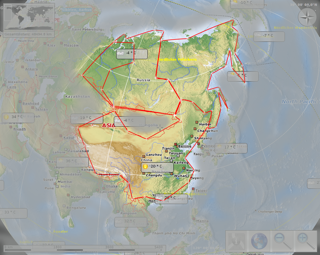
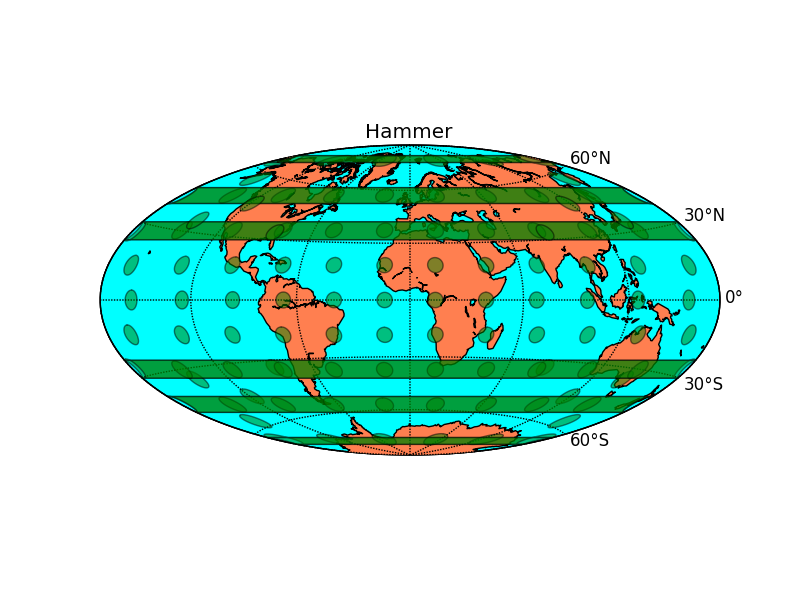
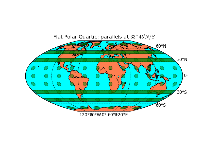
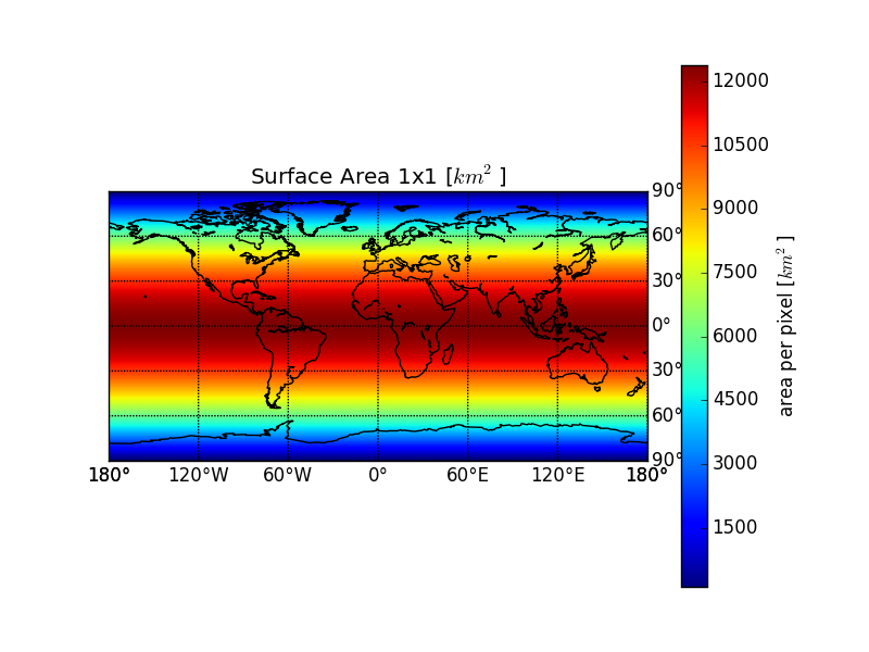
Plotting global equal area maps with python, matplotlib/pylab and Basemap.
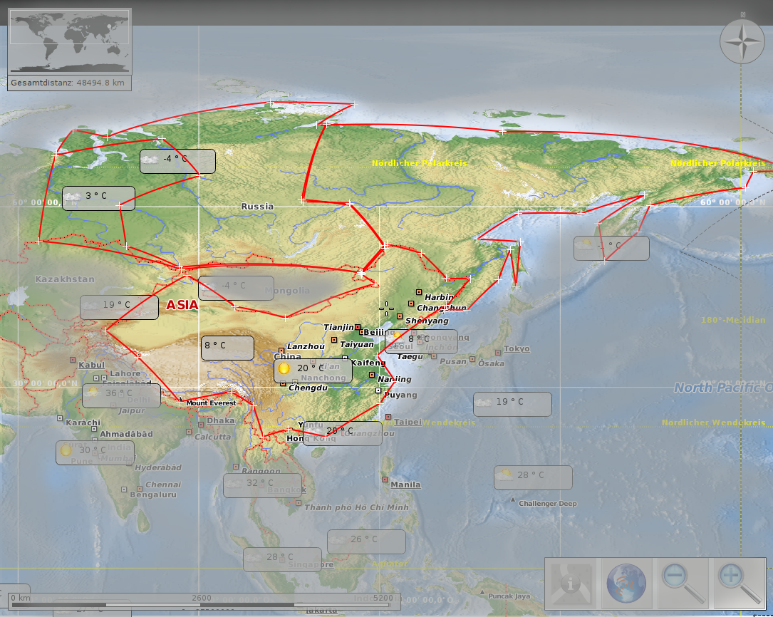
Sibiria 13,1 · 106 km² vs. china 9.7 · 106 km²
Maps thanks to Marble Desktop Globe [48] and Open Street Map [49], available under CC by-sa [50] and Open Data Commons Open Database License (ODbL) [51].
m = map.Basemap(projection='cea', lat_ts=37.5)
outfile = "hobo-dyer.png"
pl.title("Hobo Dyer: Cylindric Equal Area at $37.5^\\circ N$")
m = map.Basemap(projection='hammer', lon_0=0)
outfile = "hammer.png"
pl.title("Hammer") # latex-test: $\frac{1}{2}$
m = map.Basemap(projection='mbtfpq', lon_0=0)
outfile = "flatpolarquartic.png"
pl.title("Flat Polar Quartic: parallels at $33^\\circ 45' N/S$")
To show regional fluxes and longitudinally constrained regions: Easy to spot on rectangular grid.
To show a global overview: Helps the understanding of global data because it appears most similar to a real earth while including the whole earth surface.
For mainly latitudinally constrained regions: Straight latitudinal lines and high latitudinal resolution near the poles.
# basemap, pylab and numpy for plotting
import mpl_toolkits.basemap as map
import pylab as pl
import numpy as np
# netcdf for reading the emission files
import netCDF4 as nc
<<addmapfeatures>>
<<addindicatrix>>
try:
  <<addemissions>>
  <<addcolorbar>>
except RuntimeError: # recover from missing fluxfile
  m.fillcontinents(color='coral',lake_color='aqua')
pl.savefig(outfile)
return "./" + outfile + ""
# add map lines
m.drawcoastlines()
# only fill continents if we do not plot emissions
# m.fillcontinents(color='coral',lake_color='aqua')
m.drawparallels(np.arange(-90.,120.,30.),
                labels=[False,True,True,False])
m.drawmeridians(np.arange(0.,420.,60.),
                labels=[True,False,False,True])
m.drawmapboundary(fill_color='aqua')
# draw tissot's indicatrix to show distortion.
for y in np.linspace(m.ymax/20,19*m.ymax/20,9):
    for x in np.linspace(m.xmax/20,19*m.xmax/20,12):
        lon, lat = m(x,y,inverse=True)
        poly = m.tissot(lon,lat,4.0,100,
                        facecolor='green',
                        zorder=10,alpha=0.5)
# d = nc.Dataset("/run/media/arne/3TiB/CTDAS-2013-03-07-2years-base-data/"
#                "analysis/data_flux1x1_weekly/flux_1x1.nc")
d = nc.Dataset("UNPUBLISHED")
biocovmean = np.mean(
    d.variables["bio_flux_prior_cov"][:,:,:], axis=0)
# projection: matplotlib.org/basemap/users/examples.html
lons, lats = pl.meshgrid(range(-180, 180),
                         range(-90, 90))
x, y = m(lons, lats)
# choose my standard color range: vmin = -0.5*vmax
vmax = max(abs(np.max(biocovmean)),
           2 * abs(np.min(biocovmean)))
vmin = -0.5*vmax
m.pcolor(x, y, biocovmean, shading='flat',
         vmin=vmin, vmax=vmax) # pcolormesh is faster
pl.rcParams.update({"text.usetex": True,
                    "text.latex.unicode": True})
colorbar = pl.colorbar(orientation="horizontal",
                       format="%.2g") # scientific
colorbar.set_label("$CO_{2}$ fluxes [$\\frac{mol}{m^2 s}$]")
Emacs [57] 24.3.1 (Org [58] mode 8.0.2)
Validate XHTML 1.0 [59]
| Anhang | Größe |
|---|---|
| flatpolarquartic.png [60] | 127.57 KB |
| hobo-dyer.png [61] | 139.26 KB |
| hammer.png [62] | 138.15 KB |
| sibiria-china-flat.png [63] | 1.14 MB |
| sibiria-china-globe.png [64] | 1.14 MB |
| equal-area-map-projections.pdf [46] | 3.06 MB |
| equal-area-map-projections.org [47] | 10.19 KB |
James Hansen et al. published a paper about the expected costs due to climate change, aptly named "Young people's burden".
→ Young people's burden: requirement of negative CO2 emissions [65]
(Hansen et al. 2017, License: cc-by [66])
The paper builds on a previous paper by Hansen et al. (2016) which I summarized in Hansen 2016 got through peer-review — “Ice melt, sea level rise and superstorms” [18]. Hansen 2016 ends with many questions which need to be addressed.
Hansen 2017 says in the abstract:
We show that global temperature has risen well out of the Holocene range and Earth is now as warm as it was during the prior (Eemian) interglacial period, when sea level reached 6–9 m higher than today. Further, Earth is out of energy balance with present atmospheric composition, implying that more warming is in the pipeline, and we show that the growth rate of greenhouse gas climate forcing has accelerated markedly in the past decade.
In short: We knew for 35 years that this is coming,1 and we failed at stopping it. Now we have to fight hard to avoid the worst of the expected fallout.
However it keeps a sliver of hope to avoid the global chaos which would be likely to ensue when most coastal cities would become flooded and hundreds of millions of people would need to relocate:
Keeping warming to less than 1.5 °C or CO₂ below 350 ppm now requires extraction of CO₂ from the air. If rapid phaseout of fossil fuel emissions begins soon, most extraction can be via improved agricultural and forestry practices.
Climate Impact of Increasing Atmospheric Carbon Dioxide J. Hansen, D. Johnson, A. Lacis, S. Lebedeff, P. Lee, D. Rind, G. Russell, NASA Institute for Space Studies, Goddard Space Flight Center, 1981 [67]. Abstract: The global temperature rose by 0.2°C between the middle 1960's and 1980, yielding a warming of 0.4°C in the past century. This temperature increase is consistent with the calculated greenhouse effect due to measured increases of atmospheric carbon dioxide. Variations of volcanic aerosols and possibly solar luminosity appear to be primary causes of observed fluctuations about the mean trend of increasing temperature. It is shown that the anthropogenic carbon dioxide warming should emerge from the noise level of natural climate variability by the end of the century, and there is a high probability of warming in the 1980's. Potential effects on climate in the 21st century include the creation of drought-prone regions in North America and central Asia as part of a shifting of climatic zones, erosion of the West Antarctic ice sheet with a consequent worldwide rise in sea level, and opening of the fabled Northwest Passage. ↩
| Anhang | Größe |
|---|---|
| hansen2017--001.png [68] | 820.94 KB |
Samantha Cristoforetti reads the Hitchhikers Guide to the Galaxy on the International Space Station
This is the world we live in: The Hitchhikers Guide read from Space.
If you don’t get goosebumps just thinking about it, envision it again: The old visions are becoming real step by step, and now those who actually venture in space read the works of visionaries from their temporary home beyond the atmosphere.
New traditions form from a reality which still seems unreal.
The Hitchhikers Guide read from Space.
And yes, we had a towel with us when the kids and I went riding their scooters yesterday. We used it to dry ourselves when we came back from the rain.
I wonder when I should start reading them the Hitchhikers Guide…
I repeatedly stumbled over needing bibtex entries for the IPCC reports. So I guess, others might stumble over that, too. Here I share my bibtex entries for some parts of the IPCC reports.1
@BOOK{IPCC1990Science,
  title = {Climate Change 1990 The Science of Climate Change},
  publisher = {The Intergovernmental Panel on Climate Change},
  year = {1996},
  editor = {J.T. Houghton and G.J. Jenkins and J.J. Ephraums},
  author = {IPCC Working Group I}
}
@BOOK{IPCC1995Science,
  title = {Climate Change 1995 The Science of Climate Change},
  publisher = {The Intergovernmental Panel on Climate Change},
  year = {1996},
  editor = {J.T. Houghton and L.G. Meira Filho and B.A. Callander and N. Harris
    and A. Kattenberg and K. Maskell},
  author = {IPCC Working Group I}
}
@book{IPCCWG1PhysicalStocker2013,
   author = {IPCC},
   title = {Climate Change 2013: The Physical Science Basis. Contribution of Working Group I to the Fifth Assessment Report of the Intergovernmental Panel on Climate Change},
   publisher = {Cambridge University Press},
   address = {Cambridge, United Kingdom and New York, NY, USA},
   pages = {1535},
   ISBN = {ISBN 978-1-107-66182-0},
   DOI = {10.1017/CBO9781107415324},
   url = {www.climatechange2013.org},
   year = {2013},
   type = {Book}
}

@inbook{IPCCPolicymakersStocker2013,
   author = {IPCC},
   title = {Summary for Policymakers},
   booktitle = {Climate Change 2013: The Physical Science Basis. Contribution of Working Group I to the Fifth Assessment Report of the Intergovernmental Panel on Climate Change},
   editor = {Stocker, T.F. and Qin, D. and Plattner, G.-K. and Tignor, M. and Allen, S.K. and Boschung, J. and Nauels, A. and Xia, Y. and Bex, V. and Midgley, P.M.},
   publisher = {Cambridge University Press},
   address = {Cambridge, United Kingdom and New York, NY, USA},
   chapter = {SPM},
   pages = {1–30},
   ISBN = {ISBN 978-1-107-66182-0},
   DOI = {10.1017/CBO9781107415324.004},
   url = {www.climatechange2013.org},
   year = {2013},
   type = {Book Section}
}

@inbook{IPCCSummaryStocker2013,
   author = {Stocker, T.F. and Qin, D. and Plattner, G.-K. and Alexander, L.V. and Allen, S.K. and Bindoff, N.L. and Bréon, F.-M. and Church, J.A. and Cubasch, U. and Emori, S. and Forster, P. and Friedlingstein, P. and Gillett, N. and Gregory, J.M. and Hartmann, D.L. and Jansen, E. and Kirtman, B. and Knutti, R. and Krishna Kumar, K. and Lemke, P. and Marotzke, J. and Masson-Delmotte, V. and Meehl, G.A. and Mokhov, I.I. and Piao, S. and Ramaswamy, V. and Randall, D. and Rhein, M. and Rojas, M. and Sabine, C. and Shindell, D. and Talley, L.D. and Vaughan, D.G. and Xie, S.-P.},
   title = {Technical Summary},
   booktitle = {Climate Change 2013: The Physical Science Basis. Contribution of Working Group I to the Fifth Assessment Report of the Intergovernmental Panel on Climate Change},
   editor = {Stocker, T.F. and Qin, D. and Plattner, G.-K. and Tignor, M. and Allen, S.K. and Boschung, J. and Nauels, A. and Xia, Y. and Bex, V. and Midgley, P.M.},
   publisher = {Cambridge University Press},
   address = {Cambridge, United Kingdom and New York, NY, USA},
   chapter = {TS},
   pages = {33–115},
   ISBN = {ISBN 978-1-107-66182-0},
   DOI = {10.1017/CBO9781107415324.005},
   url = {www.climatechange2013.org},
   year = {2013},
   type = {Book Section}
}

@inbook{IPCCIntroductionCubash2013,
   author = {Cubasch, U. and Wuebbles, D. and Chen, D. and Facchini, M.C. and Frame, D. and Mahowald, N. and Winther, J.-G.},
   title = {Introduction},
   booktitle = {Climate Change 2013: The Physical Science Basis. Contribution of Working Group I to the Fifth Assessment Report of the Intergovernmental Panel on Climate Change},
   editor = {Stocker, T.F. and Qin, D. and Plattner, G.-K. and Tignor, M. and Allen, S.K. and Boschung, J. and Nauels, A. and Xia, Y. and Bex, V. and Midgley, P.M.},
   publisher = {Cambridge University Press},
   address = {Cambridge, United Kingdom and New York, NY, USA},
   chapter = {1},
   pages = {119–158},
   ISBN = {ISBN 978-1-107-66182-0},
   DOI = {10.1017/CBO9781107415324.007},
   url = {www.climatechange2013.org},
   year = {2013},
   type = {Book Section}
}

@inbook{IPCCObservationsAtmosphereSurfaceHartmann2013,
   author = {Hartmann, D.L. and Klein Tank, A.M.G. and Rusticucci, M. and Alexander, L.V. and Br\"onnimann, S. and Charabi, Y. and Dentener, F.J. and Dlugokencky, E.J. and Easterling, D.R. and Kaplan, A. and Soden, B.J. and Thorne, P.W. and Wild, M. and Zhai, P.M.},
   title = {Observations: Atmosphere and Surface},
   booktitle = {Climate Change 2013: The Physical Science Basis. Contribution of Working Group I to the Fifth Assessment Report of the Intergovernmental Panel on Climate Change},
   editor = {Stocker, T.F. and Qin, D. and Plattner, G.-K. and Tignor, M. and Allen, S.K. and Boschung, J. and Nauels, A. and Xia, Y. and Bex, V. and Midgley, P.M.},
   publisher = {Cambridge University Press},
   address = {Cambridge, United Kingdom and New York, NY, USA},
   chapter = {2},
   pages = {159–254},
   ISBN = {ISBN 978-1-107-66182-0},
   DOI = {10.1017/CBO9781107415324.008},
   url = {www.climatechange2013.org},
   year = {2013},
   type = {Book Section}
}

@inbook{IPCCObservationsOceanRhein2013,
   author = {Rhein, M. and Rintoul, S.R. and Aoki, S. and Campos, E. and Chambers, D. and Feely, R.A. and Gulev, S. and Johnson, G.C. and Josey, S.A. and Kostianoy, A. and Mauritzen, C. and Roemmich, D. and Talley, L.D. and Wang, F.},
   title = {Observations: Ocean},
   booktitle = {Climate Change 2013: The Physical Science Basis. Contribution of Working Group I to the Fifth Assessment Report of the Intergovernmental Panel on Climate Change},
   editor = {Stocker, T.F. and Qin, D. and Plattner, G.-K. and Tignor, M. and Allen, S.K. and Boschung, J. and Nauels, A. and Xia, Y. and Bex, V. and Midgley, P.M.},
   publisher = {Cambridge University Press},
   address = {Cambridge, United Kingdom and New York, NY, USA},
   chapter = {3},
   pages = {255–316},
   ISBN = {ISBN 978-1-107-66182-0},
   DOI = {10.1017/CBO9781107415324.010},
   url = {www.climatechange2013.org},
   year = {2013},
   type = {Book Section}
}

@inbook{IPCCObservationsCryosphereVaughan2013,
   author = {Vaughan, D.G. and Comiso, J.C. and Allison, I. and Carrasco, J. and Kaser, G. and Kwok, R. and Mote, P. and Murray, T. and Paul, F. and Ren, J. and Rignot, E. and Solomina, O. and Steffen, K. and Zhang, T.},
   title = {Observations: Cryosphere},
   booktitle = {Climate Change 2013: The Physical Science Basis. Contribution of Working Group I to the Fifth Assessment Report of the Intergovernmental Panel on Climate Change},
   editor = {Stocker, T.F. and Qin, D. and Plattner, G.-K. and Tignor, M. and Allen, S.K. and Boschung, J. and Nauels, A. and Xia, Y. and Bex, V. and Midgley, P.M.},
   publisher = {Cambridge University Press},
   address = {Cambridge, United Kingdom and New York, NY, USA},
   chapter = {4},
   pages = {317–382},
   ISBN = {ISBN 978-1-107-66182-0},
   DOI = {10.1017/CBO9781107415324.012},
   url = {www.climatechange2013.org},
   year = {2013},
   type = {Book Section}
}

@inbook{IPCCPaleoclimateArchivesMasson-Delmotte2013,
   author = {Masson-Delmotte, V. and Schulz, M. and Abe-Ouchi, A. and Beer, J. and Ganopolski, A. and González Rouco, J.F. and Jansen, E. and Lambeck, K. and Luterbacher, J. and Naish, T. and Osborn, T. and Otto-Bliesner, B. and Quinn, T. and Ramesh, R. and Rojas, M. and Shao, X. and Timmermann, A.},
   title = {Information from Paleoclimate Archives},
   booktitle = {Climate Change 2013: The Physical Science Basis. Contribution of Working Group I to the Fifth Assessment Report of the Intergovernmental Panel on Climate Change},
   editor = {Stocker, T.F. and Qin, D. and Plattner, G.-K. and Tignor, M. and Allen, S.K. and Boschung, J. and Nauels, A. and Xia, Y. and Bex, V. and Midgley, P.M.},
   publisher = {Cambridge University Press},
   address = {Cambridge, United Kingdom and New York, NY, USA},
   chapter = {5},
   pages = {383–464},
   ISBN = {ISBN 978-1-107-66182-0},
   DOI = {10.1017/CBO9781107415324.013},
   url = {www.climatechange2013.org},
   year = {2013},
   type = {Book Section}
}

@inbook{IPCCCarbonCycleAndOthersCiais2013,
   author = {Ciais, P. and Sabine, C. and Bala, G. and Bopp, L. and Brovkin, V. and Canadell, J. and Chhabra, A. and DeFries, R. and Galloway, J. and Heimann, M. and Jones, C. and Le Quéré, C. and Myneni, R.B. and Piao, S. and Thornton, P.},
   title = {Carbon and Other Biogeochemical Cycles},
   booktitle = {Climate Change 2013: The Physical Science Basis. Contribution of Working Group I to the Fifth Assessment Report of the Intergovernmental Panel on Climate Change},
   editor = {Stocker, T.F. and Qin, D. and Plattner, G.-K. and Tignor, M. and Allen, S.K. and Boschung, J. and Nauels, A. and Xia, Y. and Bex, V. and Midgley, P.M.},
   publisher = {Cambridge University Press},
   address = {Cambridge, United Kingdom and New York, NY, USA},
   chapter = {6},
   pages = {465–570},
   ISBN = {ISBN 978-1-107-66182-0},
   DOI = {10.1017/CBO9781107415324.015},
   url = {www.climatechange2013.org},
   year = {2013},
   type = {Book Section}
}

@inbook{IPCCCloudsAeorosolsBoucher2013,
   author = {Boucher, O. and Randall, D. and Artaxo, P. and Bretherton, C. and Feingold, G. and Forster, P. and Kerminen, V.-M. and Kondo, Y. and Liao, H. and Lohmann, U. and Rasch, P. and Satheesh, S.K. and Sherwood, S. and Stevens, B. and Zhang, X.Y.},
   title = {Clouds and Aerosols},
   booktitle = {Climate Change 2013: The Physical Science Basis. Contribution of Working Group I to the Fifth Assessment Report of the Intergovernmental Panel on Climate Change},
   editor = {Stocker, T.F. and Qin, D. and Plattner, G.-K. and Tignor, M. and Allen, S.K. and Boschung, J. and Nauels, A. and Xia, Y. and Bex, V. and Midgley, P.M.},
   publisher = {Cambridge University Press},
   address = {Cambridge, United Kingdom and New York, NY, USA},
   chapter = {7},
   pages = {571–658},
   ISBN = {ISBN 978-1-107-66182-0},
   DOI = {10.1017/CBO9781107415324.016},
   url = {www.climatechange2013.org},
   year = {2013},
   type = {Book Section}
}

@inbook{IPCCRadiativeForcingMyhre2013,
   author = {Myhre, G. and Shindell, D. and Bréon, F.-M. and Collins, W. and Fuglestvedt, J. and Huang, J. and Koch, D. and Lamarque, J.-F. and Lee, D. and Mendoza, B. and Nakajima, T. and Robock, A. and Stephens, G. and Takemura, T. and Zhang, H.},
   title = {Anthropogenic and Natural Radiative Forcing},
   booktitle = {Climate Change 2013: The Physical Science Basis. Contribution of Working Group I to the Fifth Assessment Report of the Intergovernmental Panel on Climate Change},
   editor = {Stocker, T.F. and Qin, D. and Plattner, G.-K. and Tignor, M. and Allen, S.K. and Boschung, J. and Nauels, A. and Xia, Y. and Bex, V. and Midgley, P.M.},
   publisher = {Cambridge University Press},
   address = {Cambridge, United Kingdom and New York, NY, USA},
   chapter = {8},
   pages = {659–740},
   ISBN = {ISBN 978-1-107-66182-0},
   DOI = {10.1017/CBO9781107415324.018},
   url = {www.climatechange2013.org},
   year = {2013},
   type = {Book Section}
}

@inbook{IPCCClimateModelsFlato2013,
   author = {Flato, G. and Marotzke, J. and Abiodun, B. and Braconnot, P. and Chou, S.C. and Collins, W. and Cox, P. and Driouech, F. and Emori, S. and Eyring, V. and Forest, C. and Gleckler, P. and Guilyardi, E. and Jakob, C. and Kattsov, V. and Reason, C. and Rummukainen, M.},
   title = {Evaluation of Climate Models},
   booktitle = {Climate Change 2013: The Physical Science Basis. Contribution of Working Group I to the Fifth Assessment Report of the Intergovernmental Panel on Climate Change},
   editor = {Stocker, T.F. and Qin, D. and Plattner, G.-K. and Tignor, M. and Allen, S.K. and Boschung, J. and Nauels, A. and Xia, Y. and Bex, V. and Midgley, P.M.},
   publisher = {Cambridge University Press},
   address = {Cambridge, United Kingdom and New York, NY, USA},
   chapter = {9},
   pages = {741–866},
   ISBN = {ISBN 978-1-107-66182-0},
   DOI = {10.1017/CBO9781107415324.020},
   url = {www.climatechange2013.org},
   year = {2013},
   type = {Book Section}
}

@inbook{IPCCDetectionAttributionBindoff2013,
   author = {Bindoff, N.L. and Stott, P.A. and AchutaRao, K.M. and Allen, M.R. and Gillett, N. and Gutzler, D. and Hansingo, K. and Hegerl, G. and Hu, Y. and Jain, S. and Mokhov, I.I. and Overland, J. and Perlwitz, J. and Sebbari, R. and Zhang, X.},
   title = {Detection and Attribution of Climate Change: from Global to Regional},
   booktitle = {Climate Change 2013: The Physical Science Basis. Contribution of Working Group I to the Fifth Assessment Report of the Intergovernmental Panel on Climate Change},
   editor = {Stocker, T.F. and Qin, D. and Plattner, G.-K. and Tignor, M. and Allen, S.K. and Boschung, J. and Nauels, A. and Xia, Y. and Bex, V. and Midgley, P.M.},
   publisher = {Cambridge University Press},
   address = {Cambridge, United Kingdom and New York, NY, USA},
   chapter = {10},
   pages = {867–952},
   ISBN = {ISBN 978-1-107-66182-0},
   DOI = {10.1017/CBO9781107415324.022},
   url = {www.climatechange2013.org},
   year = {2013},
   type = {Book Section}
}

@inbook{IPCCNeartermProjectionsKirtman2013,
   author = {Kirtman, B. and Power, S.B. and Adedoyin, J.A. and Boer, G.J. and Bojariu, R. and Camilloni, I. and Doblas-Reyes, F.J. and Fiore, A.M. and Kimoto, M. and Meehl, G.A. and Prather, M. and Sarr, A. and Schär, C. and Sutton, R. and van Oldenborgh, G.J. and Vecchi, G. and Wang, H.J.},
   title = {Near-term Climate Change: Projections and Predictability},
   booktitle = {Climate Change 2013: The Physical Science Basis. Contribution of Working Group I to the Fifth Assessment Report of the Intergovernmental Panel on Climate Change},
   editor = {Stocker, T.F. and Qin, D. and Plattner, G.-K. and Tignor, M. and Allen, S.K. and Boschung, J. and Nauels, A. and Xia, Y. and Bex, V. and Midgley, P.M.},
   publisher = {Cambridge University Press},
   address = {Cambridge, United Kingdom and New York, NY, USA},
   chapter = {11},
   pages = {953–1028},
   ISBN = {ISBN 978-1-107-66182-0},
   DOI = {10.1017/CBO9781107415324.023},
   url = {www.climatechange2013.org},
   year = {2013},
   type = {Book Section}
}

@inbook{IPCCLongtermProjectionsCollins2013,
   author = {Collins, M. and Knutti, R. and Arblaster, J. and Dufresne, J.-L. and Fichefet, T. and Friedlingstein, P. and Gao, X. and Gutowski, W.J. and Johns, T. and Krinner, G. and Shongwe, M. and Tebaldi, C. and Weaver, A.J. and Wehner, M.},
   title = {Long-term Climate Change: Projections, Commitments and Irreversibility},
   booktitle = {Climate Change 2013: The Physical Science Basis. Contribution of Working Group I to the Fifth Assessment Report of the Intergovernmental Panel on Climate Change},
   editor = {Stocker, T.F. and Qin, D. and Plattner, G.-K. and Tignor, M. and Allen, S.K. and Boschung, J. and Nauels, A. and Xia, Y. and Bex, V. and Midgley, P.M.},
   publisher = {Cambridge University Press},
   address = {Cambridge, United Kingdom and New York, NY, USA},
   chapter = {12},
   pages = {1029–1136},
   ISBN = {ISBN 978-1-107-66182-0},
   DOI = {10.1017/CBO9781107415324.024},
   url = {www.climatechange2013.org},
   year = {2013},
   type = {Book Section}
}

@inbook{IPCCSeaLevelChurch2013,
   author = {Church, J.A. and Clark, P.U. and Cazenave, A. and Gregory, J.M. and Jevrejeva, S. and Levermann, A. and Merrifield, M.A. and Milne, G.A. and Nerem, R.S. and Nunn, P.D. and Payne, A.J. and Pfeffer, W.T. and Stammer, D. and Unnikrishnan, A.S.},
   title = {Sea Level Change},
   booktitle = {Climate Change 2013: The Physical Science Basis. Contribution of Working Group I to the Fifth Assessment Report of the Intergovernmental Panel on Climate Change},
   editor = {Stocker, T.F. and Qin, D. and Plattner, G.-K. and Tignor, M. and Allen, S.K. and Boschung, J. and Nauels, A. and Xia, Y. and Bex, V. and Midgley, P.M.},
   publisher = {Cambridge University Press},
   address = {Cambridge, United Kingdom and New York, NY, USA},
   chapter = {13},
   pages = {1137–1216},
   ISBN = {ISBN 978-1-107-66182-0},
   DOI = {10.1017/CBO9781107415324.026},
   url = {www.climatechange2013.org},
   year = {2013},
   type = {Book Section}
}

@inbook{IPCCClimatePhenomenaChristensen2013,
   author = {Christensen, J.H. and Krishna Kumar, K. and Aldrian, E. and An, S.-I. and Cavalcanti, I.F.A. and de Castro, M. and Dong, W. and Goswami, P. and Hall, A. and Kanyanga, J.K. and Kitoh, A. and Kossin, J. and Lau, N.-C. and Renwick, J. and Stephenson, D.B. and Xie, S.-P. and Zhou, T.},
   title = {Climate Phenomena and their Relevance for Future Regional Climate Change},
   booktitle = {Climate Change 2013: The Physical Science Basis. Contribution of Working Group I to the Fifth Assessment Report of the Intergovernmental Panel on Climate Change},
   editor = {Stocker, T.F. and Qin, D. and Plattner, G.-K. and Tignor, M. and Allen, S.K. and Boschung, J. and Nauels, A. and Xia, Y. and Bex, V. and Midgley, P.M.},
   publisher = {Cambridge University Press},
   address = {Cambridge, United Kingdom and New York, NY, USA},
   chapter = {14},
   pages = {1217–1308},
   ISBN = {ISBN 978-1-107-66182-0},
   DOI = {10.1017/CBO9781107415324.028},
   url = {www.climatechange2013.org},
   year = {2013},
   type = {Book Section}
}

@inbook{IPCCannex1projectionsStocker2013,
   author = {IPCC},
   title = {Annex I: Atlas of Global and Regional Climate Projections },
   booktitle = {Climate Change 2013: The Physical Science Basis. Contribution of Working Group I to the Fifth Assessment Report of the Intergovernmental Panel on Climate Change},
   editor = {Stocker, T.F. and Qin, D. and Plattner, G.-K. and Tignor, M. and Allen, S.K. and Boschung, J. and Nauels, A. and Xia, Y. and Bex, V. and Midgley, P.M.},
   publisher = {Cambridge University Press},
   address = {Cambridge, United Kingdom and New York, NY, USA},
   chapter = {AI},
   pages = {1311–1394},
   ISBN = {ISBN 978-1-107-66182-0},
   DOI = {10.1017/CBO9781107415324.029},
   url = {www.climatechange2013.org},
   year = {2013},
   type = {Book Section}
}

@inbook{IPCCannex2scenariosStocker2013,
   author = {IPCC},
   title = {Annex II: Climate System Scenario Tables },
   booktitle = {Climate Change 2013: The Physical Science Basis. Contribution of Working Group I to the Fifth Assessment Report of the Intergovernmental Panel on Climate Change},
   editor = {Stocker, T.F. and Qin, D. and Plattner, G.-K. and Tignor, M. and Allen, S.K. and Boschung, J. and Nauels, A. and Xia, Y. and Bex, V. and Midgley, P.M.},
   publisher = {Cambridge University Press},
   address = {Cambridge, United Kingdom and New York, NY, USA},
   chapter = {AII},
   pages = {1395–1446},
   ISBN = {ISBN 978-1-107-66182-0},
   DOI = {10.1017/CBO9781107415324.030},
   url = {www.climatechange2013.org},
   year = {2013},
   type = {Book Section}
}

@inbook{IPCCannex3glossaryStocker2013,
   author = {IPCC},
   title = {Annex III: Glossary},
   booktitle = {Climate Change 2013: The Physical Science Basis. Contribution of Working Group I to the Fifth Assessment Report of the Intergovernmental Panel on Climate Change},
   editor = {Stocker, T.F. and Qin, D. and Plattner, G.-K. and Tignor, M. and Allen, S.K. and Boschung, J. and Nauels, A. and Xia, Y. and Bex, V. and Midgley, P.M.},
   publisher = {Cambridge University Press},
   address = {Cambridge, United Kingdom and New York, NY, USA},
   chapter = {AIII},
   pages = {1447–1466},
   ISBN = {ISBN 978-1-107-66182-0},
   DOI = {10.1017/CBO9781107415324.031},
   url = {www.climatechange2013.org},
   year = {2013},
   type = {Book Section}
}

@inbook{IPCCannex4acronymsStocker2013,
   author = {IPCC},
   title = {Annex IV: Acronyms},
   booktitle = {Climate Change 2013: The Physical Science Basis. Contribution of Working Group I to the Fifth Assessment Report of the Intergovernmental Panel on Climate Change},
   editor = {Stocker, T.F. and Qin, D. and Plattner, G.-K. and Tignor, M. and Allen, S.K. and Boschung, J. and Nauels, A. and Xia, Y. and Bex, V. and Midgley, P.M.},
   publisher = {Cambridge University Press},
   address = {Cambridge, United Kingdom and New York, NY, USA},
   chapter = {AIV},
   pages = {1467–1476},
   ISBN = {ISBN 978-1-107-66182-0},
   DOI = {10.1017/CBO9781107415324},
   url = {www.climatechange2013.org},
   year = {2013},
   type = {Book Section}
}

@inbook{IPCCannex5contributorsStocker2013,
   author = {IPCC},
   title = {Annex V: Contributors to the IPCC WGI Fifth Assessment Report},
   booktitle = {Climate Change 2013: The Physical Science Basis. Contribution of Working Group I to the Fifth Assessment Report of the Intergovernmental Panel on Climate Change},
   editor = {Stocker, T.F. and Qin, D. and Plattner, G.-K. and Tignor, M. and Allen, S.K. and Boschung, J. and Nauels, A. and Xia, Y. and Bex, V. and Midgley, P.M.},
   publisher = {Cambridge University Press},
   address = {Cambridge, United Kingdom and New York, NY, USA},
   chapter = {AV},
   pages = {1477–1496},
   ISBN = {ISBN 978-1-107-66182-0},
   DOI = {10.1017/CBO9781107415324},
   url = {www.climatechange2013.org},
   year = {2013},
   type = {Book Section}
}

@inbook{IPCCannex6reviewersStocker2013,
   author = {IPCC},
   title = {Annex VI: Expert Reviewers of the IPCC WGI Fifth Assessment Report},
   booktitle = {Climate Change 2013: The Physical Science Basis. Contribution of Working Group I to the Fifth Assessment Report of the Intergovernmental Panel on Climate Change},
   editor = {Stocker, T.F. and Qin, D. and Plattner, G.-K. and Tignor, M. and Allen, S.K. and Boschung, J. and Nauels, A. and Xia, Y. and Bex, V. and Midgley, P.M.},
   publisher = {Cambridge University Press},
   address = {Cambridge, United Kingdom and New York, NY, USA},
   chapter = {AVI},
   pages = {1497–1522},
   ISBN = {ISBN 978-1-107-66182-0},
   DOI = {10.1017/CBO9781107415324},
   url = {www.climatechange2013.org},
   year = {2013},
   type = {Book Section}
}

@inbook{IPCCIndexStocker2013,
   author = {IPCC},
   title = {Index},
   booktitle = {Climate Change 2013: The Physical Science Basis. Contribution of Working Group I to the Fifth Assessment Report of the Intergovernmental Panel on Climate Change},
   editor = {Stocker, T.F. and Qin, D. and Plattner, G.-K. and Tignor, M. and Allen, S.K. and Boschung, J. and Nauels, A. and Xia, Y. and Bex, V. and Midgley, P.M.},
   publisher = {Cambridge University Press},
   address = {Cambridge, United Kingdom and New York, NY, USA},
   chapter = {Index},
   pages = {1523–1535},
   ISBN = {ISBN 978-1-107-66182-0},
   DOI = {10.1017/CBO9781107415324},
   url = {www.climatechange2013.org},
   year = {2013},
   type = {Book Section}
}
In IPCC 2013 WG1 they finally provide bibtex in their zip of references [69], but without item headers — you can’t use these directly. ↩
I just made the colors of my plotting framework safe for colorblind people (thanks to Paul Tol’s notes [70]) and I want to share a very nice result I got: How to make the really websafe colors [71] safe for colorblind people with minimal changes.
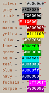
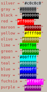
(the colorblind-safe colors are on the left, the original websafe colors on the right)
To do so, I turned to Color Oracle [72] (for simulation of colorblindness directly on my screen) and Emacs [73] rainbow-mode [74] (for seeing the colors while editing the hex-codes - as shown in the screenshots above) and tweaked the color codes bit by bit, until they were distinguishable in the simulation of Deuteranopia, Protanopia and Tritanopia.
The result were the following colorcodes:
| silver | #c0c0c0 |
| gray | #808080 |
| black | #000000 |
| red | #ff0000 |
| maroon | #800000 |
| yellow | #ffff00 |
| olive | #707030 |
| lime | #00ee00 |
| green | #009000 |
| aqua | #00eeee |
| teal | #00a0a0 |
| blue | #0000ff |
| navy | #000080 |
| fuchsia | #ff00ff |
| purple | #900090 |
The changes in detail:
- olive = "#808000"
+ olive = "#707030"

- lime = "#00ff00"
+ lime = "#00ee00"

- aqua = "#00ffff"
+ aqua = "#00eeee"

- green = "#008000"
+ green = "#009000"

- teal = "#008080"
+ teal = "#00a0a0"

- purple = "#800080"
+ purple = "#900090"
Unchanged colors: Silver, Gray, Black, Red, Maroon, Yellow, Blue, Navy, Fuchsia (and naturally White).
Caveeat: Naturally this change makes the colors less websafe, but they still stay close to their counterparts, so simple designs which use these colors can be adjusted without disrupting the visual appearance. Also this change provides a nice, small rainbow-color palette which works for colorblind people. I use it for coloring lines and symbols in plots. Being not safe for colorblind people is a sad design failure of the websafe colors - and as such of displays in general - because as I show in this article, a small adjustment to the colors would have made them safe for colorblind people. In an ideal world, the browser-developers would now come together and decide on a standard for display of these colors, so that they also become completely websafe. In the non-ideal world we live in, I’ll just specify the colors by hexcode, because accessibility trumps design.
Disclaimer: I’m not a usability or accessibility expert. I just do what I can to make my works accessible to people. If you find errors in this article or want to suggest improvements, please contact me [75].
| Anhang | Größe |
|---|---|
| websafe-colorblind-safe.png [76] | 14.65 KB |
| websafe-not-colorblindsafe.png [77] | 14.51 KB |
Calculating the area of arbitrary regions on the Earth approximated as an ellipsoid. I needed this for conversion between the output of different models.
It’s calculated in Emacs [81] Lisp, which showed me that for somewhat complex mathematical tasks Lisp syntax isn’t only unproblematic, but actually helps avoiding mistakes. And full unicode support is great for implementing algorithms with ω, λ and φ.
For converting between fluxes and emissions I need the area of arbitrary regions made up of longitude×latitude pixels - specifically the transcom regions.
But the earth is no exact sphere, but rather an oblate spheroid. I need to estimate how exact I have to calculate to keep the representation errors of the regions insignificant compared to the uncertainties of the fluxes I work with.
http://de.wikipedia.org/wiki/Erdfigur [82] http://de.wikipedia.org/wiki/Erdellipsoid [83]
„Dadurch nimmt der Meeresspiegel genähert die Form eines Rotationsellipsoids an, dessen Halbachsen (Radien) sich um 21,38 km unterscheiden (a = 6378,139 ± 0,003 km ⁽¹⁾ [84], bzw. b = 6356,752 km)“
\begin{equation} f = \frac{a-b}{a} = 1:298.25642 \pm 0.00001 \end{equation}— IERS Conventions (2003) [85].
To estimate the errors, just calculate the area of a few samples with different latitude and compare them.
Latitudes
Area-Sidelength:
The simplest case for the latitude-longitude rectangle with latitude theta, longitude phi and earth radius \( R \) looks in linear approximation like this:
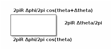
Using a cylindrical equal area rectangle projection (Lambert) we can calculate the area of a given latitude-longitude square as follows:
With θ as longitude, φ as latitude and \( R \) as radius of the earth sphere.
For a 1°×1° square, that equals
(defun spherecutarea (latdeg sidelength deglen)
  "Calculate the area of a cut in a sphere at the latitude LATDEG
with the given SIDELENGTH and the length of one degree at the
Equator DEGLEN."
  (* deglen sidelength ; longitude
     deglen sidelength (cos (* 2 float-pi (/ latdeg 360.0))))) ; latitude

(defun spherearea (latdeg sidelength)
  "Area of a segment of a sphere at LATDEG with the given
SIDELENGTH."
  (let* ((R 6371.0) ; km
         (deglen (/ (* 2 float-pi R) 360.0))) ; km^2
    (spherecutarea latdeg sidelength deglen)))
| latitude ↓ | 0.1 | 1 | 4 |
|---|---|---|---|
| 0 | 123.64 | 12364.31 | 197828.99 |
| 10 | 121.76 | 12176.47 | 194823.52 |
| 30 | 107.08 | 10707.81 | 171324.93 |
| 60 | 61.82 | 6182.16 | 98914.49 |
| 85 | 10.78 | 1077.62 | 17241.93 |
(defun spheresegmentarea (latdeg sidelength)
  "Calculate the area of a rectangular segment on a sphere at
latitude LATDEG with the given SIDELENGTH."
  (* 24728.6234228 sidelength sidelength
     (cos (* float-pi (/ latdeg 180.0)))))
spheresegmentarea
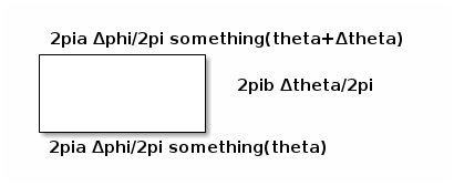
Instead of the very simple spherical compression, we can use integration over the area of an oblated spheroid, or more exactly: an ellipsoid of revolution.
An oblated spheroid has one short axis and two long axi. For the earth, the short axis is the polar radius \( b = 6356,752 km \) while the long axi have the length of the equatorial radius \( a = a = 6378,139 ± 0,003 km \).
Thus the linear approximation of an area on the spheroid looks like this:
Let’s scrap that. I’m drowning in not-so-simple ideas, so I’d rather take a pre-generated formula, even if it means cutting leafs with a chainsaw. Let’s go to an astronomy book: Astronomische Algorithmen by Jean Meeus has a formula for distances on an ellipsoid.
Taking the algorithm from Astronomische Algorithmen rev. 2 by Jean Meeus. I want to know how big the errors are when I just take a circle. So let’s implement a fitting algorithm.
The following algorithm gives us the distance between two points.
\begin{equation} F = \frac{\phi_1 + \phi_2}{2}, G = \frac{\phi_1 - \phi_2}{2}, \lambda = \frac{L_1 - L_2}{2} \end{equation} \begin{equation} S = sin^2 G ~ cos^2 G + cos^2 F ~ sin^2 \lambda \end{equation} \begin{equation} C = cos^2 G ~ cos^2 G + sin^2 F ~ sin^2 \lambda \end{equation} \begin{equation} tan \omega = \sqrt{\frac{S}{C}} \end{equation} \begin{equation} R = \frac{\sqrt{SC}}{\omega} , ~ omega ~ in ~ radians \end{equation} \begin{equation} D = 2 \omega a \end{equation} \begin{equation} H_1 = \frac{3R - 1}{2C}, H_2 = \frac{3R + 2}{2S} \end{equation} \begin{equation} s = D(1 + fH_1 ~ sin^2 F ~ cos^2 G - fH_2 ~ cos^2 F ~ sin^2 G) \end{equation}We can now use the distance \( s \) between the 4 corners of a pseudo-rectangular area on the ellipsoid to approximate the area of the pseudo-square they delimit.
\begin{equation} A = \frac{s_{bottomright - bottomleft} + s_{topright - topleft}}{2} \cdot s_{topleft - bottomleft} \end{equation}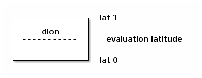
But by doing so we treat the non-linear problem as linear. To minimize the error, we can split an area into many smaller areas and sum up their areas (numerical approximation).
In following we will use the direct algorithm as well as the numerical approximation.
(defmacro turntofloatsingle (var)
  (list 'setq var (list 'float var)))

(defmacro turntofloat (&rest vars)
  "Turn a list of items to floats."
  (cons 'progn (mapcar
                (lambda (var)
                  (list 'turntofloatsingle var))
                vars)))
(defun ellipsoiddistance (a f L1 L2 φ1 φ2)
  "Calculate the distance of two arbitrary points on an ellipsoid.

  Parameters: Equator radius A, oblateness F and for point 1 and
  2 respectively the longitudes L1 and L2 and the latitudes φ1
  and φ2."
  ; ensure that we work on floats
  (turntofloat a f φ1 φ2 L1 L2)
  ; the first simplifications don’t depend on each other,
  ; so we just use let to bind them
  (let ((F (/ (+ φ1 φ2) 2))
        (G (/ (- φ1 φ2) 2))
        (λ (/ (- L1 L2) 2)))
    (message (format "F %f G %f λ %f a %f f %f L1 %f L2 %f φ1 %f φ2 %f"
                     F G λ a f L1 L2 φ1 φ2))
    ; the second don’t depend on each other either
    (let ((S (+ (* (expt (sin G) 2)
                   (expt (cos λ) 2))
                (* (expt (cos F) 2)
                   (expt (sin λ) 2))))
          (C (+ (* (expt (cos G) 2)
                   (expt (cos λ) 2))
                (* (expt (sin F) 2)
                   (expt (sin λ) 2)))))
      ; now we have a few consecutive definitions, so we use let*
      ; which allows references to previous elements in the same let*.
      (let* ((ω (atan (sqrt (/ S C))))
             (R (/    (sqrt (* S C)) ω)))
        (let ((D (* 2 ω a))
              (H1 (/ (- (* 3 R)) (* 2 C)))
              (H2 (/ (+ (* 3 R)) (* 2 C))))
          ; All prepared. Now we just fit all this together. This is
          ; the last line, so the function returns the value.
          (* D (-
                (+ 1 (* f H1 (expt (sin F) 2) (expt (cos G) 2)))
                (* f H2 (expt (cos F) 2) (expt (sin G) 2)))))))))
(defun ellipsoidrectanglearea (a f longitude latitude dlon dlat)
  (let ((L1 longitude)
        (L2 (+ longitude dlon))
        (φ1 latitude)
        (φ2 (+ latitude dlat)))
    (let ((lenlower (ellipsoiddistance a f L1 L2 φ1 φ1))
          (lenupper (ellipsoiddistance a f L1 L2 φ2 φ2))
          (lenwestern (ellipsoiddistance a f L1 L1 φ1 φ2))
          (leneastern (ellipsoiddistance a f L2 L2 φ1 φ2)))
      (if (not (= lenwestern leneastern))
          (error "Western and Eastern length are not equal.
This violates the laws of geometry. We die. Western: %f Eastern: %f"
                 lenwestern leneastern))
      (let ((horizontalmean (/ (+ lenlower lenupper) 2)))
        ; now just return length times width
        (* horizontalmean lenwestern)))))
<<ellipsoid-helpers>>
<<ellipsoid-distance>>
<<ellipsoid-rectanglearea>>

(defun ellipsoidrectangleareafromdeg (latdeg sidelength)
  "Calculate the rectangle area from the latitude LATDEG and the
SIDELENGTH given as degrees."
  (message (format "latdeg %f sidelength %f" latdeg sidelength))
  (let ((londeg 15) ; irrelevant due to symmetry
        (dlondeg sidelength)
        (dlatdeg sidelength)
        (a 6378.139)
        (f (/ 1 298.25642)))
    (let ((lon (* 2 float-pi (/ londeg 360.0))) ; 2π / 360
          (dlon (* 2 float-pi (/ dlondeg 360.0)))
          (lat (* 2 float-pi (/ latdeg 360.0)))
          (dlat (* 2 float-pi (/ dlatdeg 360.0))))
      (ellipsoidrectanglearea a f lon lat dlon dlat))))

(defun ellipsoidrectangleareafromdegnumericalintegration (latdeg sidelength steps)
  "Calculate the rectangle area from the latidute LATDEG and the
  SIDELENGTH given as degrees by adding them in STEPS smaller steps per sidelength."
  (let ((area 0)
        (smallerside (/ (float sidelength)
                        (float steps))))
    (loop for i from 0 to (1- steps) by 1 do
          (message (format "i %f" i))
          (let ((smallerlat (+ latdeg (* smallerside i))))
            ; add stepts times the area since the longitudinal
            ; calculation does not change, so we only need to
            ; calculate in once.
            (setq area (+ area (* steps
                                  (ellipsoidrectangleareafromdeg
                                   smallerlat smallerside))))))

    area))
; no return value
nil
| latitude ↓ | 0.1 | 1 | 4 |
|---|---|---|---|
| 0 | 123.9203 | 12391.0741 | 198026.1548 |
| 10 | 121.9815 | 12179.9838 | 193733.6082 |
| 20 | 116.2724 | 11592.4962 | 183457.2705 |
| 30 | 106.9937 | 10649.2503 | 167557.9088 |
| 40 | 94.4643 | 9382.6379 | 146580.1726 |
| 45 | 87.1079 | 8640.9234 | 134399.3469 |
| 50 | 79.1019 | 7834.8158 | 121219.4843 |
| 60 | 61.4002 | 6055.4408 | 92285.3707 |
| 70 | 41.9067 | 4099.4608 | 60666.5036 |
| 80 | 21.2036 | 2025.2137 | 27301.2374 |
| 85 | 10.5861 | 962.5255 | 10264.8590 |
| 90 | 0.1071 | 107.0494 | 6844.8700 |
| latitude ↓ | 0.1 | 1 | 4 |
|---|---|---|---|
| 0 | 123.9203 | 12391.3918 | 198107.5151 |
| 10 | 121.9815 | 12180.3007 | 193814.7025 |
| 20 | 116.2724 | 11592.8099 | 183537.3359 |
| 30 | 106.9937 | 10649.5549 | 167635.3476 |
| 40 | 94.4643 | 9382.9239 | 146652.3820 |
| 45 | 87.1079 | 8641.1954 | 134467.6868 |
| 50 | 79.1019 | 7835.0702 | 121283.0172 |
| 60 | 61.4002 | 6055.6486 | 92336.3892 |
| 70 | 41.9067 | 4099.6076 | 60701.4093 |
| 80 | 21.2036 | 2025.2881 | 27317.3197 |
| 85 | 10.5862 | 962.5611 | 10270.9364 |
| 90 | 0.1071 | 107.0533 | 6848.9244 |
| latitude ↓ | 0.1 | 1 | 4 |
|---|---|---|---|
| 0 | 123.9203 | 12391.3950 | 198108.3283 |
| 10 | 121.9815 | 12180.3039 | 193815.5131 |
| 20 | 116.2724 | 11592.8130 | 183538.1364 |
| 30 | 106.9937 | 10649.5580 | 167636.1220 |
| 40 | 94.4643 | 9382.9268 | 146653.1043 |
| 45 | 87.1079 | 8641.1981 | 134468.3705 |
| 50 | 79.1019 | 7835.0727 | 121283.6529 |
| 60 | 61.4002 | 6055.6507 | 92336.8997 |
| 70 | 41.9067 | 4099.6090 | 60701.7587 |
| 80 | 21.2036 | 2025.2888 | 27317.4807 |
| 85 | 10.5862 | 962.5615 | 10270.9973 |
| 90 | 0.1071 | 107.0534 | 6848.9650 |
| latitude ↓ | 0.1 | 1 | 4 |
|---|---|---|---|
| 0 | 123.9203 | 12391.3950 | 198108.3365 |
| 10 | 121.9815 | 12180.3039 | 193815.5213 |
| 20 | 116.2724 | 11592.8130 | 183538.1444 |
| 30 | 106.9937 | 10649.5580 | 167636.1297 |
| 40 | 94.4643 | 9382.9268 | 146653.1115 |
| 45 | 87.1079 | 8641.1982 | 134468.3773 |
| 50 | 79.1019 | 7835.0728 | 121283.6592 |
| 60 | 61.4002 | 6055.6507 | 92336.9048 |
| 70 | 41.9067 | 4099.6090 | 60701.7621 |
| 80 | 21.2036 | 2025.2888 | 27317.4823 |
| 85 | 10.5862 | 962.5615 | 10270.9979 |
| 90 | 0.1071 | 107.0534 | 6848.9654 |
| latitude ↓ | 0.1 | 1 | 4 |
|---|---|---|---|
| 0 | 0.0000% | 0.0026% | 0.0411% |
| 10 | 0.0000% | 0.0026% | 0.0419% |
| 20 | 0.0000% | 0.0027% | 0.0436% |
| 30 | 0.0000% | 0.0029% | 0.0462% |
| 40 | 0.0000% | 0.0030% | 0.0493% |
| 45 | 0.0000% | 0.0031% | 0.0508% |
| 50 | 0.0000% | 0.0032% | 0.0524% |
| 60 | 0.0000% | 0.0034% | 0.0553% |
| 70 | 0.0000% | 0.0036% | 0.0575% |
| 80 | 0.0000% | 0.0037% | 0.0589% |
| 85 | 0.0000% | 0.0037% | 0.0592% |
| 90 | 0.0000% | 0.0037% | 0.0592% |
| latitude ↓ | 0.1 | 1 | 4 |
|---|---|---|---|
| 0 | 0.000000% | 0.000026% | 0.000410% |
| 10 | 0.000000% | 0.000026% | 0.000418% |
| 20 | 0.000000% | 0.000027% | 0.000436% |
| 30 | 0.000000% | 0.000029% | 0.000462% |
| 40 | 0.000000% | 0.000030% | 0.000493% |
| 45 | 0.000000% | 0.000031% | 0.000508% |
| 50 | 0.000000% | 0.000032% | 0.000524% |
| 60 | 0.000000% | 0.000034% | 0.000553% |
| 70 | 0.000000% | 0.000036% | 0.000576% |
| 80 | 0.000000% | 0.000037% | 0.000589% |
| 85 | 0.000000% | 0.000037% | 0.000592% |
| 90 | 0.000000% | 0.000037% | 0.000593% |
| latitude ↓ | 0.1 | 1 | 4 |
|---|---|---|---|
| 0 | 0.000000% | 0.000000% | 0.000004% |
| 10 | 0.000000% | 0.000000% | 0.000004% |
| 20 | 0.000000% | 0.000000% | 0.000004% |
| 30 | 0.000000% | 0.000000% | 0.000005% |
| 40 | 0.000000% | 0.000000% | 0.000005% |
| 45 | 0.000000% | 0.000000% | 0.000005% |
| 50 | 0.000000% | 0.000000% | 0.000005% |
| 60 | 0.000000% | 0.000000% | 0.000006% |
| 70 | 0.000000% | 0.000000% | 0.000006% |
| 80 | 0.000000% | 0.000000% | 0.000006% |
| 85 | 0.000000% | 0.000000% | 0.000006% |
| 90 | 0.000000% | 0.000000% | 0.000006% |
This is almost done in the theory. Only thing left to do: Use the algorithm to generate a list of areas per 1° latitude and pass that to a python script which writes it into a netCDF4 file for later usage.
I need a python snippet which takes a list of values from lat 0° to lat 90° as input and turns it into a 360°×180° map.
Or I could just write the data from the elisp code to a file and read that.
<<ellipsoidrectangleareafromdeg>>
(with-temp-file "transcomellipticlat90-sum1000.dat"
  ; switch to the opened file
  (switch-to-buffer (current-buffer))
  (loop for lat from 0 to 90 do
        (insert (concat (number-to-string lat) " "))
        (insert (number-to-string
                 (ellipsoidrectangleareafromdegnumericalintegration lat 1 1000)))
        (insert "\n")))
; dang, this is beautiful!
<<ellipsoidrectangleareafromdeg>>
(with-temp-file "transcomellipticlat90-direct.dat"
  ; switch to the opened file
  (switch-to-buffer (current-buffer))
  (loop for lat from 0 to 90 do
        (insert (concat (number-to-string lat) " "))
        (insert (number-to-string
                 (ellipsoidrectangleareafromdegnumericalintegration lat 1 1)))
        (insert "\n")))
<<ellipsoidrectangleareafromdeg>>
(with-temp-file "transcomellipticlat90-sum1000vsdirect.dat"
  ; switch to the opened file
  (switch-to-buffer (current-buffer))
  (loop for lat from 0 to 90 do
        (insert (concat (number-to-string lat) " "))
        (insert (number-to-string
                 (- (ellipsoidrectangleareafromdegnumericalintegration lat 1 1000)
                    (ellipsoidrectangleareafromdegnumericalintegration lat 1 1))))
        (insert "\n")))
<<ellipsoidrectangleareafromdeg>>
<<spherearea>>
(with-temp-file "transcomellipticlat90-sum1000vssphere.dat"
  ; switch to the opened file
  (switch-to-buffer (current-buffer))
  (loop for lat from 0 to 90 do
        (insert (concat (number-to-string lat) " "))
        (insert (number-to-string
                 (- (ellipsoidrectangleareafromdegnumericalintegration lat 1 1000)
                    (spherearea lat 1))))
        (insert "\n")))
<<spherearea>>
(with-temp-file "transcomellipticlat90-sphere.dat"
  ; switch to the opened file
  (switch-to-buffer (current-buffer))
  (loop for lat from 0 to 90 do
        (insert (concat (number-to-string lat) " "))
        (insert (number-to-string (spherearea lat 1)))
        (insert "\n")))
(with-temp-file "transcomellipticlat90-sum1000vssphere.dat"
  ; switch to the opened file
  (switch-to-buffer (current-buffer))
  (loop for lat from 0 to 90 do
        (insert (concat (number-to-string lat) " "))
        (insert (number-to-string (- (ellipsoidrectangleareafromdegnumericalintegration lat 1 1000) (spheresegmentarea lat 1))))
        (insert "\n")))
Now just readout that file as csv
The following codeblock can be summoned into other code via
<<addplotstyle>>
# add map lines
m.drawcoastlines()
m.drawparallels(np.arange(-90.,120.,30.),
                labels=[False,True,True,False])
m.drawmeridians(np.arange(0.,420.,60.),
                labels=[True,False,False,True])
m.drawmapboundary(fill_color='aqua')
import numpy as np
import pylab as pl
import mpl_toolkits.basemap as bm
import netCDF4 as nc
def singlehemispherelats2map(northernlats):
    """Turn the northern lats (0-90) into a map (180,360)."""
    # duplicate the northernlats
    lats = np.zeros((180, ))
    lats[0:90] = northernlats[:0:-1,1]
    lats[90:] = northernlats[1:,1]
    # and blow them up into a map
    lons = np.ones((360, ))
    lats = np.matrix(lats)
    lons = np.matrix(lons)
    mapscaling = lons.transpose() * lats
    mapscaling = mapscaling.transpose()
    return mapscaling

# first read the file
with open("transcomellipticlat90-sum1000.dat") as f:
    northernlats = np.genfromtxt(f, delimiter=" ")
mapscaling = singlehemispherelats2map(northernlats)
with open("transcomellipticlat90-sum1000vsdirect.dat") as f:
    northernlats = np.genfromtxt(f, delimiter=" ")
mapscalingdiff = singlehemispherelats2map(northernlats)
with open("transcomellipticlat90-direct.dat") as f:
    northernlats = np.genfromtxt(f, delimiter=" ")
mapscalingdirect = singlehemispherelats2map(northernlats)
with open("transcomellipticlat90-sphere.dat") as f:
    northernlats = np.genfromtxt(f, delimiter=" ")
mapscalingsphere = singlehemispherelats2map(northernlats)
with open("transcomellipticlat90-sum1000vssphere.dat") as f:
    northernlats = np.genfromtxt(f, delimiter=" ")
mapscalingdiffsphere = singlehemispherelats2map(northernlats)
# several different plots:
<<plotareamapperpixel>>
<<plotareamapperpixeldirect>>
<<plotareamapperpixelerror>>
<<plotareamapperpixelrelerror>>
<<plotareamapperpixelsphereerror>>
# plot it for representation
m = bm.Basemap()
m.imshow(mapscaling)
bar = pl.colorbar()
bar.set_label("area per pixel [$km^2$]")
<<addplotstyle>>
pl.title("Surface Area 1x1 [$km^2$]")
pl.savefig("eartharea_1x1.png")
pl.close()
print """\n\n#+caption:Area when summing 1000x1000 smaller areas
[[./eartharea_1x1.png]]"""
m = bm.Basemap()
m.imshow(mapscaling)
bar = pl.colorbar()
bar.set_label("area per pixel [$km^2$]")
# summon map style! :)
<<addplotstyle>>
pl.title("Surface Area 1x1, no numerical integration [$km^2$]")
pl.savefig("earthareadirect_1x1.png")
pl.close()
print "\n\n#+caption:Area when using just one square\n[[./earthareadirect_1x1.png]]"
m = bm.Basemap()
m.imshow(mapscalingdiff)
<<addplotstyle>>
bar = pl.colorbar()
bar.set_label("area per pixel [$km^2$]")
pl.title("Surface Area 1x1 difference: sum 1000 vs direct [$km^2$]")
pl.savefig("eartharea1000vs1_1x1.png")  # save as a clean netCDF4 file
pl.close()
print "\n\n#+caption:Difference between summing smaller squares",
print "and just using one square\n[[./eartharea1000vs1_1x1.png]]"
m = bm.Basemap()
m.imshow(np.log(np.abs(mapscalingdiff/mapscaling)))
<<addplotstyle>>
bar = pl.colorbar()
bar.set_label("relative error per pixel, logarithmic")
pl.title("Surface Area 1x1 diff relative: sum 1000 vs direct")
pl.savefig("eartharea1000vs1rel_1x1.png")  # save as a clean netCDF4 file
pl.close()
print """\n\n#+caption:Relative Area Error by not integrating (logscale)
[[./eartharea1000vs1rel_1x1.png]]"""
m = bm.Basemap()
m.imshow(np.log(np.abs(mapscalingdiffsphere/mapscaling)))
<<addplotstyle>>
bar = pl.colorbar()
bar.set_label("relative error per pixel, logarithmic")
pl.title("Surface Area 1x1 diff relative: sum 1000 vs sphere")
pl.savefig("eartharea1000vssphererel_1x1.png")
pl.close()
print """\n\n#+caption:Relative Error from Sphere (logscale)
[[./eartharea1000vssphererel_1x1.png]]"""
<<readcsvareafiles>>
<<plotareamaps>>
D = nc.Dataset("eartharea.nc", "w")
D.comment = "Created with tm5tools/ct2pyshell/transcomareas.org"
D.createDimension("longitude", 360)
D.createDimension("latitude", 180)
area = D.createVariable("1x1", "f8", ("latitude", "longitude"))
area.units = "km^2"
area.comment = "from 180W to 180E and from 90S to 90N"
area[:] = mapscaling
area = D.createVariable("1x1_1000vs1", "f8", ("latitude", "longitude"))
area.units = "km^2"
area.comment = ("Difference between the direct calculation of the "
"area and summing up 1000x1000 smaller areas."
"from 180W to 180E and from 90S to 90N")
area[:] = mapscalingdiff
area = D.createVariable("1x1_direct", "f8", ("latitude", "longitude"))
area.units = "km^2"
area.comment = ("Area calculated without numerical intergration (bigger errors!). "
"from 180W to 180E and from 90S to 90N")
area[:] = mapscalingdirect
area = D.createVariable("1x1_sphere", "f8", ("latitude", "longitude"))
area.units = "km^2"
area.comment = ("Area calculated on a simple sphere. "
"from 180W to 180E and from 90S to 90N")
area[:] = mapscalingsphere
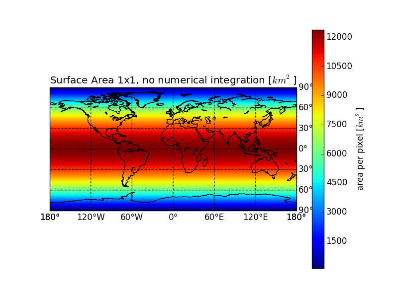
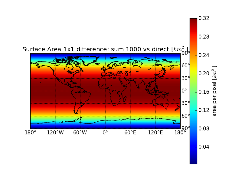
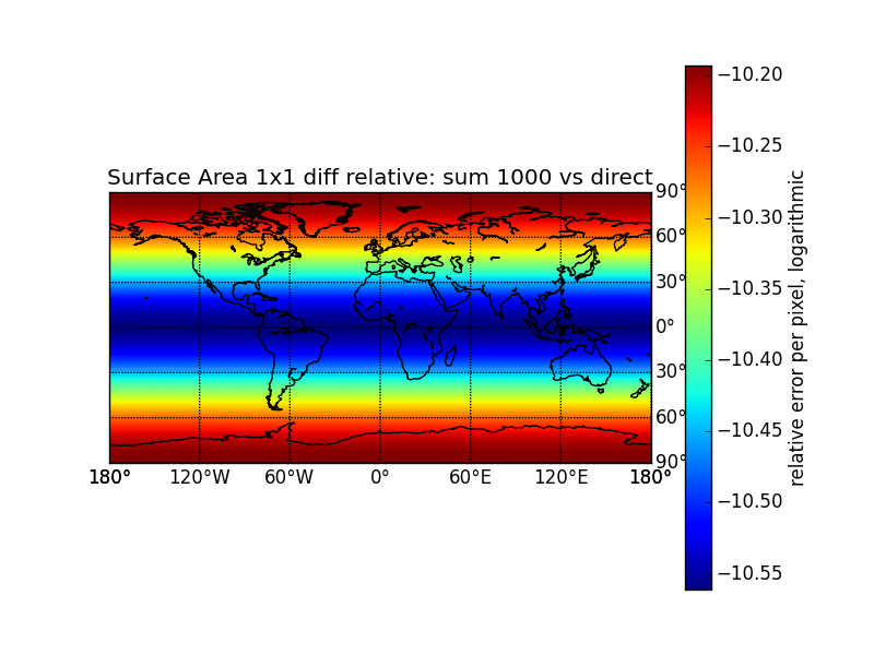
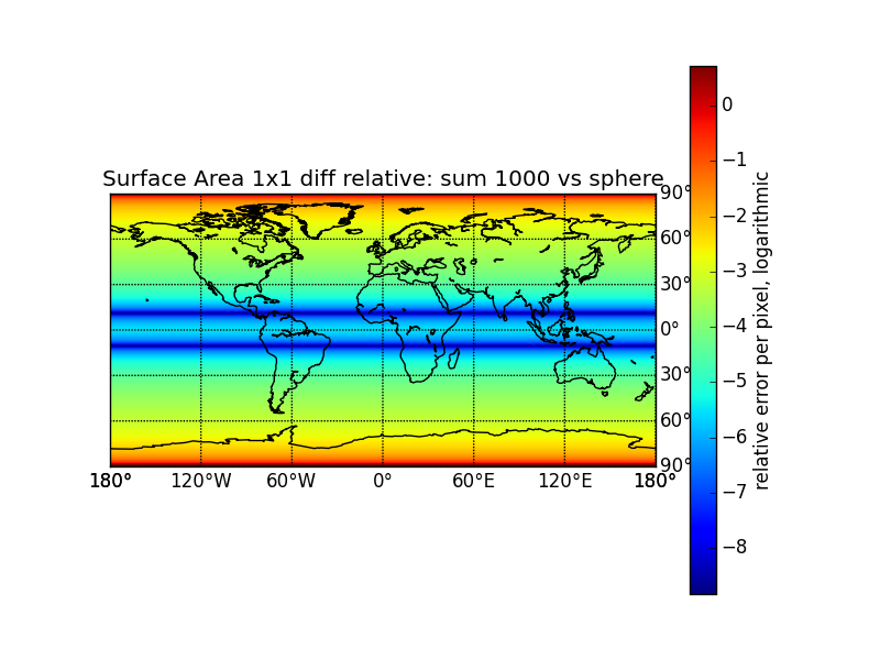
Should be around 510 million km²
(let ((s 0))
  (loop for lat from 0 to 90 do
        (setq s (+ s (spherearea lat 1))))
  (/ (* 2 360 s) 1.0e6)) ; million kilometers
514.5026761832414
(let ((s 0))
  (loop for lat from 0 to 90 do
        (setq s (+ s (ellipsoidrectangleareafromdegnumericalintegration lat 1 1))))
  (/ (* 2 360 s) 1.0e6)) ; million kilometers
509.55872913305257
(let ((s 0))
  (loop for lat from 0 to 90 do
        (setq s (+ s (ellipsoidrectangleareafromdegnumericalintegration lat 1 10))))
  (/ (* 2 360 s) 1.0e6)) ; million kilometers
509.57373786401286
(let ((s 0))
  (loop for lat from 0 to 90 do
        (setq s (+ s (ellipsoidrectangleareafromdegnumericalintegration lat 1 1000))))
  (/ (* 2 360 s) 1.0e6)) ; million kilometers
509.5738894527161
Should be around 7,692,024 km² + 269,652 km² = 7,961,676 km²
import netCDF4 as nc
import numpy as np
import pylab as pl

D = nc.Dataset("eartharea.nc")
area = D.variables["1x1"][:]
T = nc.Dataset("../plotting/transcom_regions_ct/regions.nc")
transcom = T.variables["transcom_regions"][:]
mask = transcom[::-1,:] == 10
pl.imshow(mask*area)
bar = pl.colorbar()
bar.set_label("area per pixel [$km^2$]")
pl.title("Area of Australia and New Zealand in [$km^2$] per pixel")
pl.savefig("area-australia.png")
# pl.show()
return np.sum(mask*area)
7976938.58492
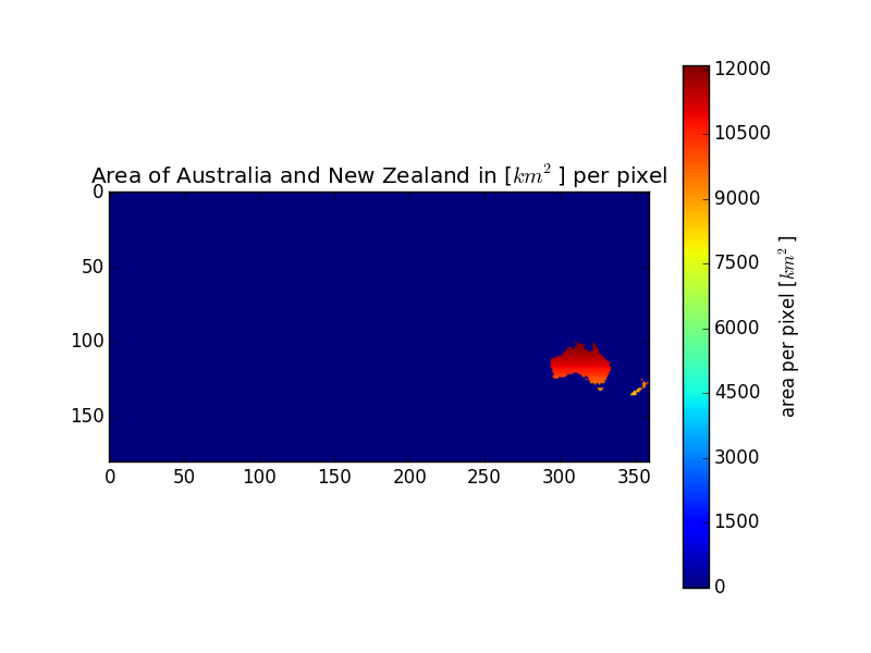
Figure 1: Area of Australia and New Zealand
The area of 1x1 degree pixels on a worldmap in ellipsoid approximation is available in the file eartharea.nc [80] in the variable “1x1”. Visualized it looks like this:
Figure 2: Surface Area of the Earth in \(km^2\)
To calculate the emissions from mol/m², just multiply each gridpoint with 106 m²/km² and the gridpoint in the variable:
<<prep>>
import numpy as np
import pylab as pl
import mpl_toolkits.basemap as bm
import netCDF4 as nc
D = nc.Dataset("eartharea.nc")
area = D.variables["1x1"][:]
flux = np.ones((180, 360)) * np.random.normal(0.0, 1.e-6, (180, 360))
emiss = flux*area
m = bm.Basemap()
m.imshow(emiss)
<<addplotstyle>>
bar = pl.colorbar()
bar.set_label("emissions [mol/s]")
pl.title("random flux $0 \pm 1.e-6 \\frac{mol}{m^{2}s}$ turned to random emissions")
filename = "randomemissions.png"
pl.savefig(filename)
print "#+caption: Random emissions in simple lat/lon plot."
print "[[./" +  filename + "]]"
# plot again, with hobo-dyer projection (equal-area)
pl.close()
m = plotmap(emiss)
<<addplotstyle>>
bar = pl.colorbar()
bar.set_label("emissions [mol/s]")
pl.title("random emissions in hobo-dyer projection")
filename = "randomemissionshobo-dyer.png"

pl.savefig(filename)
print """\n\n#+caption: Random Emissions in Hobo Dyer Projection
[[./""" +  filename + "]]"
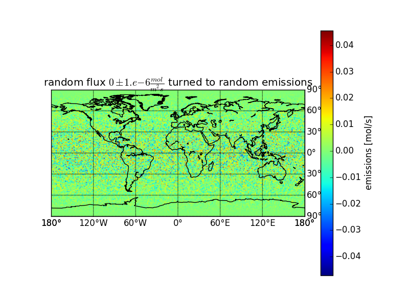
Figure 3: Random emissions in simple lat/lon plot.
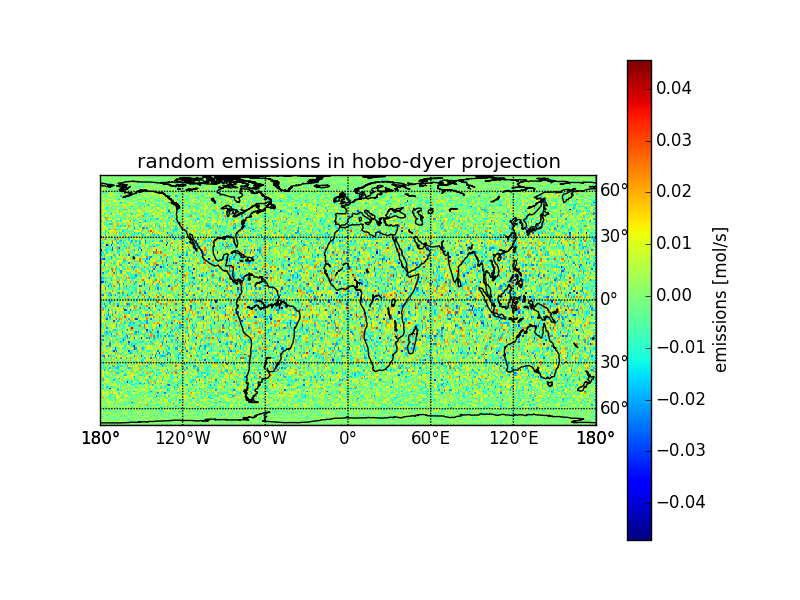
Figure 4: Random Emissions in Hobo Dyer Projection
def plotmap(array):
    """Plot an array as map."""
    m = bm.Basemap(projection='cea', lat_ts=37.5)
    ny, nx = array.shape[:2]
    lons, lats = pl.meshgrid(range(-nx/2, nx/2 + nx%2),
                             range(-ny/2, ny/2 + ny%2))
    x, y = m(lons, lats)
    arr = array.copy()
    for i in arr.shape[2:]:
        arr = arr[:,:,0]
    m.pcolormesh(x, y, arr)
    return m
Estimating the land area for a given lat-lon region (this requires a
land/sea map in the file t3_regions_landsea.nc, i.e. from TM5-4DVar,
see tm5.sf.net [88]).
<<prep>>
import netCDF4 as nc
import numpy as np
import pylab as pl
import mpl_toolkits.basemap as bm


def landarea(lat0, lon0, lat1, lon1):
    """Calculate the land area in the rectangle defined by the
    arguments.

    :param lat0: latitude in degree. Southern Hemisphere negative.
    :param lon0: longitude in degree. East negative.

    :returns: landarea within the rectangle in km^2

    >>> samarea = 17.840 * 1000000 # km^2
    >>> ae = landarea(15, -90, -60, -30)
    >>> 0.99 * samarea < ae < 1.01 * samarea
    True
    """
    lat0idx = int(lat0 + 90)
    lat1idx = int(lat1 + 90)
    if lat0idx > lat1idx:
        tmp = lat1idx
        lat1idx = lat0idx
        lat0idx = tmp
    lon0idx = int(lon0 + 180)
    lon1idx = int(lon1 + 180)
    if lon0idx > lon1idx:
        tmp = lon1idx
        lon1idx = lon0idx
        lon0idx = tmp
    D = nc.Dataset("eartharea.nc")
    T = nc.Dataset("t3_regions_landsea.nc")
    area = D.variables["1x1"][:]
    landfraction05x05 = T.variables["LSMASK"][:]
    landfraction1x1 = np.zeros((180,360)) # latxlon
    for i in range(landfraction1x1.shape[0]):
        for j in range(landfraction1x1.shape[1]):
            landfraction1x1[i,j] = np.mean(landfraction05x05[i*2:i*2+2,:][:,j*2:j*2+2])
    landarea = area * landfraction1x1
    # m = plotmap(landfraction1x1)
    # pl.show()
    # m = plotmap(landarea)
    # pl.show()
    return np.sum(landarea[lat0idx:lat1idx+1,:][:,lon0idx:lon1idx])


if True or __name__ == "__main__":
    import doctest
    doctest.testmod()
Most of the code snippets here are thanks to ggole in #emacs on irc.freenode.net (What is IRC? [89]).
(defmacro turntofloatsingle (var)
  (list 'setq var (list 'float var)))
<<turntofloat-single>>
(defmacro turntofloatbackticks (&rest vars)
  "Turn a list of items to floats using backtick notation."
  `(progn ,@(mapcar
             (lambda (var)
               `(turntofloatsingle ,var))
             vars)))
<<turntofloat-single>>
(defmacro turntofloat (&rest vars)
  "Turn a list of items to floats (without using backticks)."
  ; cons turns this into a call of progn on the list returned by
  ; mapcar
  (cons 'progn (mapcar
                (lambda (var)
                  (list 'turntofloatsingle var))
                vars)))
<<turntofloat-single>>
(defmacro turntofloatcollect (&rest vars)
  "Turn a list of items to floats, using the collect directive of loop."
  ; execute progn on the list returned by the loop
  (cons 'progn
        ; loop ... collect returns a list of all the loop results.
        (loop for var in vars collect
              (list 'turntofloatsingle var))))
<<turntofloat-single>>

; build the list explicitely to make it easier for me to understand
; what the macro does
(defmacro turntofloatexplicit (&rest vars)
  "Turn a list of items to floats (using explicit list building
instead of mapcar)."
  ; prepare an empty list of function calls
  (let ((funclist '()))
    ; for each variable add a call to the single-item macro
    (loop for var in vars do
          ; (list 'turntofloatsingle var) creates the call to
          ; turntofloatsingle with the variable which is referenced by
          ; var. Push puts that at the beginning of the funclist.
          (push (list 'turntofloatsingle var) funclist))
    ; to ensure the right order of operations, we reverse the funclist
    (setq funclist (reverse funclist))
    ; cons turns this into a call of progn on the list. We need progn,
    ; because the funclist contains multiple function calls.
    (cons 'progn funclist)))
<<turntofloat-single>>
; Common Lisp Macro to turn the place to a float in one step.
(defmacro turntofloatinline (&rest places)
  "Turn a list of items to floats using an inline function call."
  `(progn ,@(mapcar
             (lambda (place)
               `(callf float ,place)) places)))
<<turntofloat-collect>>
(setq a 1 b 3.8 c 2)
(turntofloatcollect a b c)
(message (number-to-string c))
| Anhang | Größe |
|---|---|
| eartharea-eartharea_1x1.png [90] | 88.19 KB |
| eartharea.nc [80] | 1.98 MB |
| eartharea.pdf [78] | 1.19 MB |
| eartharea-area-australia.png [91] | 33.3 KB |
| eartharea-eartharea1000vs1_1x1.png [92] | 86.35 KB |
| eartharea-eartharea1000vssphererel_1x1.png [93] | 98.72 KB |
| eartharea-eartharea1000vs1rel_1x1.png [94] | 92.39 KB |
| eartharea-eartharea_1x1.png [95] | 88.19 KB |
| eartharea-earthareadirect_1x1.png [96] | 90.13 KB |
| eartharea-randomemissions.png [97] | 353.01 KB |
| eartharea-randomemissionshobo-dyer.png [98] | 239.52 KB |
| eartharea-segmentellipsoid.png [99] | 5.39 KB |
| eartharea-segmentellipsoiddistances.png [100] | 2.72 KB |
| eartharea-segmentsphere.png [101] | 5.24 KB |
| eartharea.org [79] | 42.75 KB |
AGU publications published "The world's biggest gamble", a short commentary on how to go on with climate change.
I am hard pressed not to become sarcastic. Not because the commentary is wrong. It’s spot on. But because we, as a species, are …
I’ll stop speaking my mind for now. Let’s hope that hope wins against frustration and our children don’t have to pay too dearly for the idiocy of my generation and the generation before.
Oh well, Happy Halloween and enjoy Samhain.
New version: draketo.de/wissen/greenhouse-effect-calculated [103]
I did not want to talk about the greenhouse effect without having checked the math and physics. Therefore I calculated it myself.
If you want all links to work, read the the PDF-version [104].
The greenhouse effect describes the effect of the atmosphere on Earth’s surface temperature. The simplest example contrasts the surface temperature of a planet without atmosphere to the surface temperature with a single insulating layer above the surface.
The incoming radiation from the Sun provides the earth with a constant source of energy. If it would not get rid of that energy somehow, it would get hotter everyday, eventually melt and vaporize. It’s evident that this does not happen (otherwise we would not be here to think about it).
As shown by \citet{Stefan1879} and \citet{Boltzmann1884}, the total energy emission from a perfect black body (a body which absorbs all incoming radiation) per unit area is given by
\begin{equation} E = \sigma T^4 \end{equation}
with the Stefan–Boltzmann constant
\begin{equation} \sigma = \frac{2 \pi^5 k^4}{15 c^2 h^3} \approx 5.67 \cdot 10^{-8} W m^{-2} K^{-4} \end{equation}
From satellite measurements in the Earth’s orbit we know that the incident solar radiation delivers an average energy flux \(j\) between 1361 \(Wm^{-2}\) during the solar minimum and to 1363 \(Wm^{-2}\) during the solar maximum \citep{KoppSolarConstant2011}.
This radiation hits the cross section of the Earth, the area of a circle with the radius of the Earth: \(\pi R^2\). This is also the energy radiated by the Earth system, as evidenced by the Earth neither melting nor freezing. But this outgoing radiation is perpendicular to the surface, not to the cross section of the Earth. The total surface of a sphere is \(4 \times \pi R^2\), or \(4 \times\) its cross section. So the energy radiated per area is just 25% of the incoming energy: \(σT_{out}^4 = 0.25 \times σT_{in}^4\)
The incident radiation delivers an Energy flux of \(E_i = 1362 Wm^{2}\), so the outgoing radiation of a perfect black body would be \(E_o = 340.5 Wm^{-2}\), which is consistent with a temperature of
\begin{equation} T = \left(\frac{E}{σ}\right)^{\frac{1}{4}} = \left(\frac{340.5 \cdot 15 c^2 h^3}{2 \pi^5 k^4}\right)^{\frac{1}{4}} K \approx \left(\frac{340.5}{5.67 \cdot 10^{-8}}\right)^{\frac{1}{4}} K = 278.623 K \end{equation}
This gives an average surface temperature of
\begin{equation} (278.62 - 273.15) ^\circ C = 5.47 ^\circ C \end{equation}
for a perfectly black Earth without atmosphere.
Due to the simplifications used, this value is \(8 K\) lower than the measured mean sea and land surface temperature of \(14 ^\circ C\) for the base period 1961-90 \citep{Jones1999,Rayner2006}.
Historically the next step after the black body estimation was to take the albedo into account: The amount of incoming radiation reflected directly back into space.
If we take into account that the Earth surface and clouds reflect roughly 30% of the visible light back into space, the Earth only receives roughly 70% of the energy which it needs to radiate back. For details, see \citet{Muller2012} and \citet{Muller2013}.1 The equilibrium temperature changes to 255 Kelvin, which is just about -18 °C. Note that changing the albedo by 1 percent point (to 29% or 31%) would change the temperature by roughly 1 K.
(let* ((albedo 0.3)
       (sol 1362)
       (incoming-watt (* (- 1 albedo) (/ sol 4)))
       (c 3e8)
       (h 6.62607e-34)
       (k 1.38065e-23)
       (pi 3.14159))
  (expt
   (/ (* incoming-watt 15 c c (expt h 3))
      (* 2 (expt pi 5) (expt k 4)))
   0.25))
254.61953320379396
\begin{equation} T = \left(\frac{E}{σ}\right)^{\frac{1}{4}} = \left(\frac{0.7 \cdot 340.5 \cdot 15 c^2 h^3}{2 \pi^5 k^4}\right)^{\frac{1}{4}} K \approx \left(\frac{238.0}{5.67 \cdot 10^{-8}}\right)^{\frac{1}{4}} K = 254.6 K \end{equation}
There are small additional factors in play:
But with these we’re still roughly 30 Kelvin away from actual temperatures. These are reached through absorption and radial re-radiation of outgoing energy, which effectively provides the Earth with insulation, most effective in the infrared.
This is what is typically called the greenhouse effect: Infra-red emissions by the Earth are absorbed by greenhouse gases in the atmosphere, so the Earth needs to be warmer to get rid of the same amount of received energy.
Greenhouse gases have a net effect on the temperature, because the outgoing radiation mostly consists of thermal infrared light (TIR), while the incoming radiation mostly consists of near infrared (NIR) visible (VIS) and ultraviolet (UV) light. Let’s take the oldest account of this absorption: \citet[“On the Influence of Carbonic Acid in the Air upon the Temperature of the Ground”]{Arrhenius1896} describes different absorption of moonlight depending on the wavelength of the light. Half this light absorbed in the atmosphere is radiated outwards, the other half inwards.
For the actual calculation, we use more recent results: \citet[„The natural greenhouse effect of atmospheric oxygen (O2)and nitrogen (N2)“]{Hoepfner2012}. They take into account the structure of the atmosphere by building on the well-established Karlsruhe Optimized and Precise Radiative transfer Algorithm (KOPRA) [106].
The publication by \citet[]{Hoepfner2012} showed that Outgoing Longrange Radiation without gas would be 365.7 W/m\(^2\), while with greenhouse gases it is 242.7 W/m\(^2\). That’s a 33.6 % decrease in emission, so we need 1.5 times higher emissions to reach equilibrium. Let’s factor this into the equations, and also use an emissivity of 0.95.
(let* ((albedo 0.3)
       (emiss 0.95)
       (sol 1362)
       (incoming-watt (* (- 1 albedo) (/ sol 4)))
       (c 3e8)
       (h 6.62607e-34)
       (k 1.38065e-23)
       (pi 3.14159))
  (expt
   (/ (* (/ 365.7 242.7) incoming-watt (/ 1 emiss) 15 c c (expt h 3))
      (* 2 (expt pi 5) (expt k 4)))
   0.25))
       ;; for the numerator
       ;; (* (/ 365.7 242.7) (/ 1 emiss) incoming-watt))
285.7423501045961
\begin{equation} T = \left(\frac{E}{σ}\right)^{\frac{1}{4}} = \left(\frac{\frac{365.7}{242.7} \cdot 0.7\frac{1}{0.95} \cdot 340.5 \cdot 15 c^2 h^3}{2 \pi^5 k^4}\right)^{\frac{1}{4}} K \approx \left(\frac{377.49}{5.67 \cdot 10^{-8}}\right)^{\frac{1}{4}} K = 285.74 K \end{equation}
We get 285.74 K as equilibrium temperature. That’s around 12.6°C, so now we’re just 1.4 Kelvin away from the actual \(14 ^\circ C\) for the base period 1961-90 \citep{Jones1999,Rayner2006}. There are still effects missing in the calculations, but the intention of this guide is not to create a new climate model, but to show the fundamental physical effects. Remember also that changing the surface albedo by 1 percent point (to 29% or 31%) would change the temperature by roughly 1 K, so getting within less than 2 °C of the measured temperature is already pretty good. Going further would require a much stricter treatment of surface albedo that goes into too much detail for an article.
Therefore we’ll round this up with an important test that is only weakly affected by the surface albedo:
What happens if we increase the absorption by CO\(_2\)? Do we see global warming?
For this test the result is already close enough to the measured temperature that we can take the difference between values with different parameters to get the effect of these parameters and remove biases which are present in both values.
To calculate global warming due to doubled CO₂, we cannot just double the absorption, because the absorption bands get saturated. The \citet[IPCC working group 1 (physical science basis)]{IPCCRadiativeForcingMyhre2013} gives the increase in radiative forcing due to increased CO\(_2\) levels [107] from the 1950 concentrations of about 310 ppm to the 2010 concentrations of 390 ppm as about 1.2 W/m\(^2\).2
So let us go at this backwards: \citet{Hoepfner2012} showed the state for 2012, what do our calculations predict for 1950 when we reduce the absorption due to CO\(_2\) by the 1.2 W/m\(^2\) radiative forcing given in the IPCC?3
The unstable emissions would then not be 242.7 W/m\(^2\) as calculated by \citet{Hoepfner2012}, but 243.9 W/m\(^2\).
(let* ((albedo 0.3)
       (sol 1362)
       (emiss 0.95)
       (incoming-watt (* (- 1 albedo) (/ sol 4)))
       (c 3e8)
       (h 6.62607e-34)
       (k 1.38065e-23)
       (pi 3.14159))
  (expt
   (/ (* (/ 365.7 (+ 242.7 1.2)) incoming-watt (/ 1 emiss) 15 c c (expt h 3))
      (* 2 (expt pi 5) (expt k 4)))
   0.25))
       ;; for the numerator
       ;; (* (/ 365.7 (+ 242.7 1.2)) incoming-watt (/ 1 emiss)))
285.3902331695058
We get 285.39 Kelvin for 1950, about 0.35°C less than for 2010.
This gives an estimate of a 0.35°C increase in temperature from 1950 to 2010 due to increased CO\(_2\) levels alone. If we also remove the added absorption from methane, N\(_{2}O\) and other greenhouse gases emitted by humans (additional forcing of 0.75 W/m\(^2\)), we get 285.17 Kelvin.
So this calculation from basics yields an increase of the equilibrium temperature by 0.57 °C.
\begin{equation} T_{2010} - T_{1950} = 285.74 K - 285.17 K = 0.57 K \end{equation}
This is a bit lower than the increase of 0.65 K to 0.75 K seen in the global temperature records by the Berkeley Earth project [108],4 and close to the 0.6 to 0.8 K increase shown in the Global (NH+SH)/2 temperature given by HadCRUT4 by the Met Office Hadley Centre by the National Meteorological Service of the United Kingdom [109].5 But for a calculation from basic principles, that’s pretty good.
So we can conclude that actual measurements match this physical explanation of global warming due to the greenhouse effect — or more exactly: due to increased absorption of infrared radiation by greenhouse gases, with the biggest effect due to CO\(_2\).
The source of climate-active human carbon emissions which influences the CO\(_2\) content of the atmosphere is mostly burning of fossil fuel which is taken from the crust of the Earth and introduced into the carbon cycle. This is what changes the CO\(_2\) concentration.
And with this, we are done.
Please reduce your carbon emissions and become active to get politicians to action on a national and global scale. We’re cutting the branch we live on.
If you want more details, have a look at the IPCC reports. Best start with the executive summary and then go into the details you’re most interested in:
IPCC Climate Change 2013: The Physical Science Basis: https://www.ipcc.ch/report/ar5/wg1/ [110]
An explanation how humans increase the CO₂-concentration of the atmosphere is available in my presentation The carbon cycle [111]: https://www.draketo.de/licht/physik/kohlenstoffkreislauf-carbon-cycle [111]
And if you want my best estimate of our current situation, have a look at the article Two visions of our future [112]: https://www.draketo.de/english/politics/roll-a-die [112]
You can check the albedo for several different spectral regions at http://www.globalbedo.org/ [113]
Robust data about changing CO\(_2\) levels is available from the Global Monitoring Division (GMD) of the Earth System Research Laboratory (ESRL) at the National Oceanic & Atmospheric Administration (NOAA) [114].
We’re only going to 1950 and not back to 1850, because the temperature data at 1850 would mix in the effect of the declining little ice age [115].
Berkeley Earth provides a reevaluation of all the surface measurements without complex models.
HadCRUT4 combines sea surface temperature data from the Hadley Centre of the UK Met Office and the land surface air temperature records compiled by the Climatic Research Unit (CRU) of the University of East Anglia.
| Anhang | Größe |
|---|---|
| greenhouse-effect.org [105] | 20.95 KB |
| greenhouse-effect-solar-radiation-earth-radiation.svg [116] | 14.6 KB |
| greenhouse-effect-solar-radiation-earth-radiation.png [117] | 62.39 KB |
| greenhouse-effect-thumbnail.png [118] | 12.76 KB |
| greenhouse-effect.pdf [104] | 349.56 KB |
I just discussed with “sceptics” on twitter about climate change. There Ronan Connolly (@RonanConnolly) showed me his article which tries to give the impression that there is no scientific consensus about climate change being man-made. I spent some time answering that, and I want to share those answers here so they do not get lost in twittering.
This is how that started:
Ronan Connolly: @ArneBab @dhb7 @randal_olson Arne, have you read my "Is there a scientific consensus on global warming? [119]" essay? — 8:14 PM - 27 Jun 2014 [120]
These are my answers, in the short format I used on twitter, just with the recipients taken out (because those are highly repetitive):
your scale of 1 to 5 mixes up two completely separate issues: “Is it a crisis” and “is it man-made”
You later complain that people mix global warming and man-made, but that’s what you do in the article.
Your claim that modellers want to hide uncertainty is also wrong: They are up-front with uncertainties.
At this point I saw a reply from Ronan (I had missed about 5 others because I was busy actually reading the article and watching the videos linked in it):
Ronan Conolly: Did you read the Shackley et al., 1999 article I referenced as an example?
that article says that modellers don’t talk publicly about adjustments they themselves call fudge-factors which correct for stuff the models cannot represent correctly yet - and links to a 15 year old paper which scientists have since acted upon and replaced the adjustments by measures backed with solid theory [121]. To give the article of Ronan credit: It does also link to chapter in the IPCC which states that those flux adjustments are no longer used.
If you wonder why some don’t talk openly, just read your own article. I already debunked lots of it. Will you include that?
Ronan Conolly: Which bits have you debunked?
The core of my criticism (1/2): you show man-made + crisis vs. natural + harmless — and then complain people mix that up.
core criticism (2/2): You show 5 equal positions, while even Singer says “most disagree with me” ⇒ Misrepresents statistics.
You show a linear range, but there is a distribution of scientific views - with the huge majority on the man-made side.
If you give as much space for a fringe position as for a majority position, you distort the actual distribution.
You list “examples”, but actually you picked a scale and then show 2-3 on each point on the scale. Try that with racism.
and the range you show isn’t actually one range, but two distributions. Man-made is almost a consensus. Catastrophic is not.
you complain about terminology (global warming vs. man-made g.w.) and then you use a scale which mixes both together.
On Prof. John Christy: I saw some model-results this week. Models cannot yet predict regional changes.
(he claims that the regional distribution of temperature change disagrees with models, and uses that to argument that there is no global warming)
On Prof. Christy: Greenpeace showed, when cutting all subsidies wind is already cheaper than nuclear.
Ronan Connolly: 1) Can you give a reference? […]
Reference to greenpeace showing that wind and water are cheaper than coal and nuclear: greenpeace-energy.de/presse/artikel/article/wind-und-wasser-schon-heute-billiger-als-kohle-und-atom.html [122]
Debunking Prof. Carter: “half the scientists think the warming natural” ← None from the ones I know personally.
Debunking Singer: The oceans in the last 15 years show the warming. Same for satellites: http://www.skepticalscience.com/satellite-measurements-warming-troposphere.htm …
But to give Singer credit: He correctly assessed that most climate scientists disagree with him.
Also you cite Prof. Svensmark and then say the equivalent of “the base of their theory has been disproven”.
Ronan Connolly: 1) I said Svensmarck's work is hotly debated, not "disproven". 2) Do you agree that there's wide range of views on global warming?
On Svensmark: I said “it’s the equivalent of disproven”, because including new data destroys the correlation it’s based on.
(the second part was already disproven earlier in this article: Not one range, two distributions with a very clear consensus-peak at man-made)
To make the article halfways accurate in reflecting the scientific view, there are two most important points to change:
Done right (1/2): 2 scales: man-made vs. natural and crisis vs. harmless. ⇒ consistent with complaint that people mix these.
Done right (2/2): Ask scientists instead of using media interviews (distorted due to the fair-and-balanced doctrine).
(note that the fair-and-balanced doctrine is special to climate science: On Russia they never require fair-and-balanced)
(naturally the scientists have to be picked at random, so the distribution of views is sampled correctly).
Scientific institutions1 currently base a large part of their internal evaluation, their comparison to others, and their hiring decisions on counting publication (with a number of different scorings).
And this is dumb.
On the surface this causes pressure to publish as many papers as possible2 which drives down quality of publications to the lowest standard reviewers accept.3 And it strengthens a hierarchy of publishers, where some publications are worth more than others based on the name of the journal. That simplifies funding decisions. But makes them worse. And it creates an incentive to get a maximum of prestige with a minimum of substance.4
But publications are how scientists communicate. Adding another purpose to them reduces their value for communication — and as such harms the scientific process. Add to this that the number of scientists is rising and that scientific communication is already facing a scalability crisis [123], and it becomes obvious that counting publications as a metric of value is dumb. That’s clear to every scientist I ever talked to in person (there are people in online-discussions who disagree).
That it is still done shows that this pressure to publish is a symptom of an underlying problem.
This deeper problem is that there is no possible way to judge scientific quality independently. But universities and funders want competition (by ideology). Therefore they crave metrics. But »When a measure becomes a target, it ceases to be a good measure. [124]«
Science is a field where typically only up to 100 people can judge the actual quality of your work, and most of these 100 people know each other. Competition does not work as quality control in such a setting; instead, competition creates incentives for corruption and group-thinking. Therefore the only real defense against corruption are the idealism of scientific integrity (“we’re furthering human knowledge”) and harsh penalties when you get caught (you can never work as scientist again).
But if you have to corrupt your communication to be able to work in the first place, this creates perverse incentives to scientists5 and might on the long run destroy the reliability of science.
Therefore counting publications to measure success has to stop.
Science is a field in which constant competition undermines the core features society requires to derive value from it. Post-doc scientists proved over more than a decade that they want to do good work. Their personal integrity is what keeps science honest. Scientific integrity is still prevailing in most fields against the corrupting incentives from constant forced competition, but it won’t last forever.
If we as society want scientists we can trust, if we want scientific integrity, we have to move away from competition and towards giving more people permanent positions in public institutions; especially for science staff, the people who do the concrete work; the people who conduct experiments, search for mathematical proofs, and model theories.
Scientific integrity, personal motivation to do good work for the scientific sub-community (of around 100 people), and idealism (which can mean to contradict the community), along with the threat of being permanently expelled for fraud, are the drivers which produce good, reliable scientific results.
To get good, reliable results in science, the most important task is therefore to ensure that scientists do not have to worry too much about other things than their scientific integrity, their scientific community, and their idealism. Because it is only the intrinsic motivation [125] of scientists which can ensure the quality of scientific work.
For this article scientific institutions mainly means those state-actors who finance scientists and those private actors who employ scientists and compete for state funding. ↩
The problem here is pressure to inflate the impact metrics of publications. Publishing should be about communicating research, not about boosting ones job opportunities. ↩
This argument is based on discussions I had with many other scientists over the years, along with experiences like seeing that people split publications into several papers to increase the publication count, even though that does not improve the publication itself. It is also based on the realization that few scientists I met were still following all publications in their sub-field. For a longer reasoning see information challenges in scientific communication [123]. ↩
That said: While I did my PhD and postdoc in atmospheric physics (up until 2017), I worked with many scientists from several different countries, and every single one of them lived the idealism of scientific integrity and put it before the harmful incentives. So while some of the incentives over the past decades are a problem, they do not at present destroy the reliability of science in general. ↩
The effect of these perverse incentives get even worse, by the divide (keyword: dual labor market) [126] between those in secure positions and young scientists which forces almost everyone to survive the stage with perverse incentives before securing a stable position. This is so striking that from the outside it must look as if the current employment structure had been designed with the explicit intent to disrupt scientific integrity, though “grasping for straws when trying to do the impossible” (quantifying scientific quality) is likely a better explanation — which does not shed a good light on science administration and policy makers. ↩
Links:
[1] http://sn.1w6.org/group/science
[2] http://sn.1w6.org/notice/137020
[3] https://web.archive.org/web/20140904134447/http://buildfreedom.com/content/scientific_method.shtml
[4] https://www.draketo.de/deutsch/wissenschaftliche-methode
[5] http://draketo.de/comment/reply/383#comment-form
[6] https://www.draketo.de/licenses
[7] https://www.earth-syst-dynam.net/9/1085/2018/
[8] https://www.draketo.de/english/science/hansen-2017
[9] http://www.atmos-chem-phys.net/16/3761/2016/
[10] http://www.atmos-chem-phys.net/16/3761/2016/acp-16-3761-2016.pdf
[11] http://www.atmos-chem-phys.net/16/3761/2016/acp-16-3761-2016-supplement.pdf
[12] http://www.atmos-chem-phys.net/16/3761/2016/acp-16-3761-2016.bib
[13] https://www.scientificamerican.com/article/major-report-prompts-warnings-that-the-arctic-is-unraveling1/?WT.mc_id=SA_ENGYSUS_20170504
[14] https://www.amap.no/documents/doc/Snow-Water-Ice-and-Permafrost.-Summary-for-Policy-makers/1532
[15] http://www.nature.com/news/climate-science-rising-tide-1.13749
[16] https://pubs.giss.nasa.gov/abs/ha02700w.html
[17] http://www.huffingtonpost.com/dr-james-hansen/twenty-years-later-tippin_b_108766.html
[18] https://www.draketo.de/english/science/hansen-2016
[19] http://draketo.de/node/764
[20] https://osf.io/ezcuj/
[21] https://osf.io/phtye/
[22] http://www.scientificamerican.com/article/massive-international-project-raises-questions-about-the-validity-of-psychology-research/?WT.mc_id=SA_BS_20150828
[23] http://www.deutschlandfunk.de/reproduzierbarkeit-forscherkollektiv-testet-100-studien.676.de.html?dram:article_id=329589
[24] https://www.draketo.de/files/2014-11-28-Fr-information-challenges-scientific-publishing.pdf
[25] https://www.draketo.de/files/2014-11-28-Fr-information-challenges-scientific-publishing.org
[26] https://translate.google.com/translate?sl=auto&tl=en&js=y&prev=_t&hl=de&ie=UTF-8&u=http://draketo.de/licht/politik/erhaltet-eure-links&edit-text=&act=url
[27] http://draketo.de/licht/politik/erhaltet-eure-links
[28] http://journal.frontiersin.org/article/10.3389/fenvs.2014.00016/full
[29] http://www.annualreviews.org/
[30] http://www.pro-physik.de/phy/physik/journalHome.html
[31] http://www.scientificamerican.com/
[32] http://draketo.de/light/english/free-software/makefile-to-autotools
[33] https://translate.google.com/translate?sl=auto&tl=en&js=y&prev=_t&hl=de&ie=UTF-8&u=http://draketo.de/reproduzierbare-veroeffentlichungen&edit-text=&act=url
[34] http://draketo.de/reproduzierbare-veroeffentlichungen
[35] https://ogbe.net/blog/sloppy_papers.html
[36] http://gnu.org/s/automake
[37] http://microformats.org/
[38] https://www.draketo.de/zitate#measure-target
[39] https://en.wikipedia.org/wiki/Goodhart%27s_law
[40] http://biorxiv.org/content/early/2017/03/21/118356
[41] https://doi.org/10.1101/118356
[42] https://forbetterscience.com/2017/03/29/cope-the-publishers-trojan-horse-calls-to-abolish-retractions/
[43] https://www.draketo.de/english/science/challenges-scientific-publishing#sec-2-3-3
[44] http://www.draketo.de/english/science/challenges-scientific-publishing#sec-2-3-3
[45] https://www.draketo.de/files/conversion-factor-ppmv-co2-to-gtc.png
[46] https://www.draketo.de/files/equal-area-map-projections.pdf
[47] https://www.draketo.de/files/equal-area-map-projections.org
[48] http://kde.org/applications/education/marble/
[49] http://www.openstreetmap.org/
[50] http://creativecommons.org/licenses/by-sa/2.0/
[51] http://opendatacommons.org/licenses/odbl/
[52] http://onlinelibrary.wiley.com/doi/10.1029/JB078i011p01753/abstract
[53] http://matplotlib.org/basemap/
[54] http://www.scipy.org/PyLab
[55] http://www.numpy.org/
[56] http://code.google.com/p/netcdf4-python/
[57] http://www.gnu.org/software/emacs/
[58] http://orgmode.org
[59] http://validator.w3.org/check?uri=referer
[60] https://www.draketo.de/files/flatpolarquartic.png
[61] https://www.draketo.de/files/hobo-dyer.png
[62] https://www.draketo.de/files/hammer.png
[63] https://www.draketo.de/files/sibiria-china-flat.png
[64] https://www.draketo.de/files/sibiria-china-globe.png
[65] https://www.earth-syst-dynam.net/8/577/2017/
[66] https://creativecommons.org/licenses/by/3.0/
[67] http://science.sciencemag.org/content/213/4511/957
[68] https://www.draketo.de/files/hansen2017--001.png
[69] http://www.climatechange2013.org/images/uploads/WGIAR5_Citations_FinalRev1.zip
[70] http://www.sron.nl/~pault/
[71] http://en.wikipedia.org/wiki/HTML_color_names#HTML_color_names
[72] http://colororacle.org/
[73] http://gnu.org/s/emacs
[74] http://elpa.gnu.org/packages/rainbow-mode.html
[75] https://www.draketo.de/contact
[76] https://www.draketo.de/files/websafe-colorblind-safe.png
[77] https://www.draketo.de/files/websafe-not-colorblindsafe.png
[78] https://www.draketo.de/files/eartharea.pdf
[79] https://www.draketo.de/files/eartharea.org
[80] https://www.draketo.de/files/eartharea.nc
[81] https://www.draketo.de/english/emacs
[82] http://de.wikipedia.org/wiki/Erdfigur
[83] http://de.wikipedia.org/wiki/Erdellipsoid
[84] http://onlinelibrary.wiley.com/doi/10.1029/GL001i001p00035/abstract;jsessionid=937BFAA6038DDCF51FD6E7567DD5EAFB.d03t04?deniedAccessCustomisedMessage=&userIsAuthenticated=false
[85] http://www.iers.org/IERS/EN/Publications/TechnicalNotes/tn32.html
[86] http://www.stats.govt.nz/browse_for_stats/snapshots-of-nz/nz-in-profile-2013/about-new-zealand.aspx
[87] http://www.ga.gov.au/education/geoscience-basics/dimensions/area-of-australia-states-and-territories.html
[88] http://tm5.sf.net
[89] http://en.wikipedia.org/wiki/Internet_Relay_Chat
[90] https://www.draketo.de/files/eartharea-eartharea_1x1.png
[91] https://www.draketo.de/files/eartharea-area-australia.png
[92] https://www.draketo.de/files/eartharea-eartharea1000vs1_1x1.png
[93] https://www.draketo.de/files/eartharea-eartharea1000vssphererel_1x1.png
[94] https://www.draketo.de/files/eartharea-eartharea1000vs1rel_1x1.png
[95] https://www.draketo.de/files/eartharea-eartharea_1x1_0.png
[96] https://www.draketo.de/files/eartharea-earthareadirect_1x1.png
[97] https://www.draketo.de/files/eartharea-randomemissions.png
[98] https://www.draketo.de/files/eartharea-randomemissionshobo-dyer.png
[99] https://www.draketo.de/files/eartharea-segmentellipsoid.png
[100] https://www.draketo.de/files/eartharea-segmentellipsoiddistances.png
[101] https://www.draketo.de/files/eartharea-segmentsphere.png
[102] http://onlinelibrary.wiley.com/doi/10.1002/2016EF000392/pdf
[103] https://www.draketo.de/wissen/greenhouse-effect-calculated
[104] https://www.draketo.de/files/greenhouse-effect_4.pdf
[105] https://www.draketo.de/files/greenhouse-effect_4.org
[106] https://www.imk-asf.kit.edu/english/312.php
[107] https://www.ipcc.ch/report/ar5/wg1/anthropogenic-and-natural-radiative-forcing/
[108] http://berkeleyearth.org/2018-temperatures/
[109] https://www.metoffice.gov.uk/hadobs/hadcrut4/diagnostics.html
[110] https://www.ipcc.ch/report/ar5/wg1/
[111] https://www.draketo.de/licht/physik/kohlenstoffkreislauf-carbon-cycle
[112] https://www.draketo.de/english/politics/roll-a-die
[113] http://www.globalbedo.org/
[114] https://www.esrl.noaa.gov/gmd/ccgg/trends/
[115] https://en.wikipedia.org/wiki/Little_Ice_Age
[116] https://www.draketo.de/files/greenhouse-effect-solar-radiation-earth-radiation.svg
[117] https://www.draketo.de/files/greenhouse-effect-solar-radiation-earth-radiation_0.png
[118] https://www.draketo.de/files/greenhouse-effect-thumbnail.png
[119] http://globalwarmingsolved.com/2013/11/is-there-a-scientific-consensus-on-global-warming/
[120] https://twitter.com/1RonanConnolly/status/482587686314979328
[121] http://www.ipcc.ch/publications_and_data/ar4/wg1/en/ch8s8-2-7.html
[122] http://www.greenpeace-energy.de/presse/artikel/article/wind-und-wasser-schon-heute-billiger-als-kohle-und-atom.html
[123] https://www.draketo.de/english/science/challenges-scientific-publishing
[124] http://www.draketo.de/zitate#measure-target
[125] https://www.draketo.de/light/english/motivation-and-payment
[126] https://blogs.lse.ac.uk/impactofsocialsciences/2013/12/11/how-academia-resembles-a-drug-gang/