Exploring the probability of successfully retrieving a file in freenet, given different redundancies and chunk lifetimes
Table of Contents
In this text I want to explore the behaviour of the degrading yet redundant anonymous file storage in Freenet. It only applies to files which were not subsequently retrieved.
Every time you retrieve a file, it gets healed which effectively resets its timer as far as these calculations here are concerned. Due to this, popular files can and do live for years in freenet.
1 Static situation
Firstoff we can calculate the retrievability of a given file with different redundancy levels, given fixed chunk retrieval probabilities.
Files in Freenet are cut into segments which are again cut into up to 256 chunks each. With the current redundancy of 100%, only half the chunks of each segment have to be retrieved to get the whole file. I call that redundancy “2x”, because it inserts data 2x the size of the file (actually that’s just what I used in the code and I don’t want to force readers - or myself - to make mental jumps while switching from prose to code).
We know from the tests done by digger3, that after 31 days about 50% of the chunks are still retrievable, and after 30 days about 30%. Let’s look how that affects our retrieval probabilities.
# encoding: utf-8
from spielfaehig import spielfähig
from collections import defaultdict
data = []
res = []
for chunknumber in range(5, 105, 5):...
byred = defaultdict(list)
for num, prob, red, retrieval in data:...
csv = "; num prob retrieval"
for red in byred:...

# now plot the files

plotcmd = """
set term png
set width 15
set xlabel "chunk probability"
set ylabel "retrieval probability"
set output freenet-prob-redundancy-2.png
plot "2.csv" using 2:3 select ($1 == 5) title "5 chunks", "" using 2:3 select ($1 == 10) title "10 chunks", "" using 2:3 select ($1 == 30) title "30 chunks", "" using 2:3 select ($1 == 100) title "100 chunks"
set output freenet-prob-redundancy-3.png
plot "3.csv" using 2:3 select ($1 == 5) title "5 chunks", "" using 2:3 select ($1 == 10) title "10 chunks", "" using 2:3 select ($1 == 30) title "30 chunks", "" using 2:3 select ($1 == 100) title "100 chunks"
set output freenet-prob-redundancy-4.png
plot "4.csv" using 2:3 select ($1 == 5) title "5 chunks", "" using 2:3 select ($1 == 10) title "10 chunks", "" using 2:3 select ($1 == 30) title "30 chunks", "" using 2:3 select ($1 == 100) title "100 chunks"
"""
with open("plot.pyx", "w") as f:...

from subprocess import Popen
Popen(["pyxplot", "plot.pyx"])
So what does this tell us?
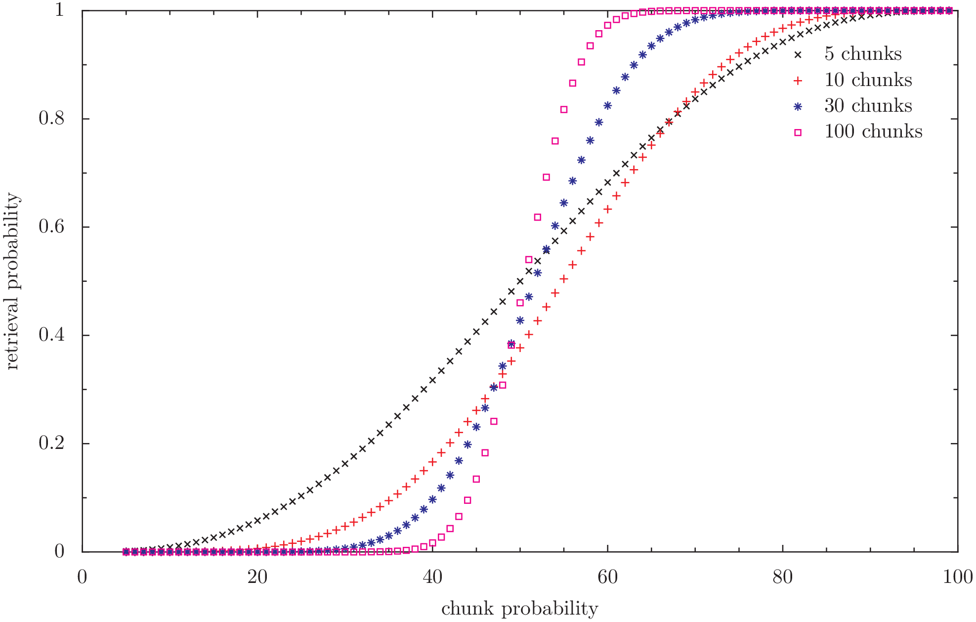
Retrieval probability of a given file in a static case. redundancy 100% (2)
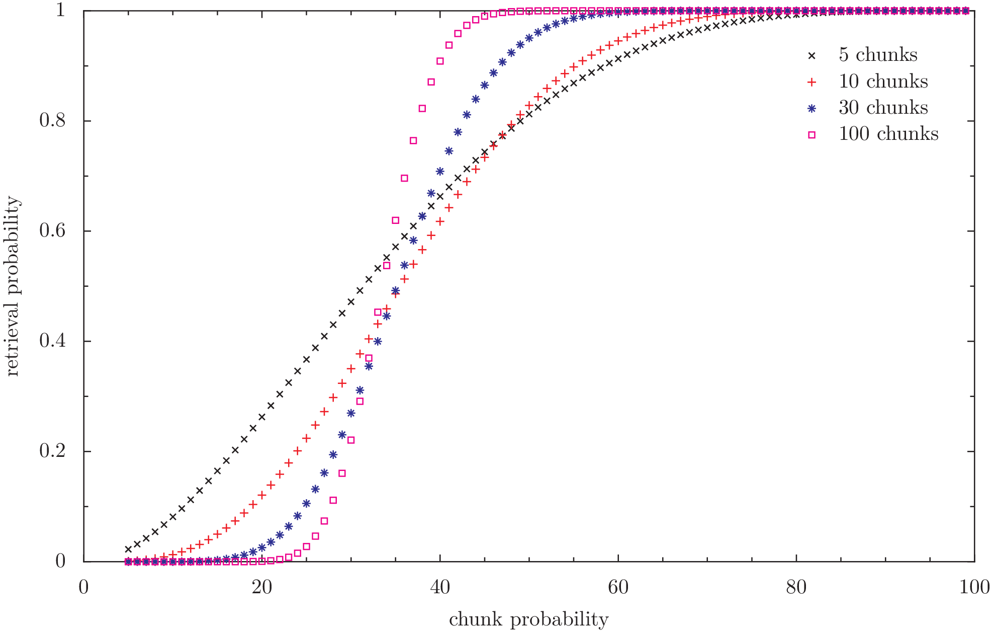
Retrieval probability of a given file in a static case. redundancy 200% (3)
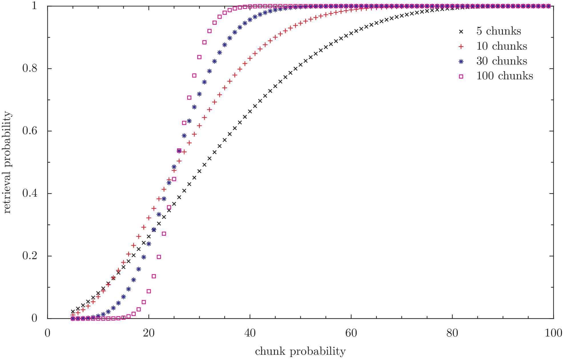
Retrieval probability of a given file in a static case. redundancy 300% (4)
This looks quite good. After all, we can push the lifetime as high as we want by just increasing redundancy.
Sadly it is also utterly wrong :) Let’s try to get closer to the real situation.
2 Dynamic Situation: The redundancy affects the replacement rate of chunks
To find a better approximation of the effects of increasing the redundancy, we have to stop looking at freenet as a fixed store and have to start seeing it as a process. More exactly: We have to look at the replacement rate.
2.1 Math
A look on the stats from digger3 shows us, that after 4 weeks 50% of the chunks are gone. Let’s call this the dropout rate. The dropout rate consists of churn and chunk replacement:
dropout = churn + replacement
Since after one day the dropout rate is about 10%, I’ll assume that the churn is lower than 10%. So for the following parts, I’ll just ignore the churn (naturally this is wrong, but since the churn is not affected by redundancy, I just take it as constant factor. It should reduce the negative impacts of increasing redundancy). So we will only look at replacement of blocks.
Replacement consists of new inserts and healing of old files.
replacement = insert + healing
If we increase the redundancy from 2 to 3, the insert and healing rate should both increase by 50%, so the replacement rate should increase by 50%, too. The healing rate might increase a bit more, because healing can now restore 66% of the file as long as at least 33% are available. I’ll ignore that, too, for the time being (which is wrong again. We will need to keep this in mind when we look at the result).
redundancy 2 → 3 ⇒ replacement rate × 1.5
Increasing the replacement rate by 50% should decrease the lifetime of chunks by 1/1.5, or:
chunk lifetime × 2/3
So we will be at the 50% limit not after 4 weeks, but after 10 days. But on the other hand, redundancy 3 only needs 33% chunk probability, which has 2× the lifetime of 50% chunk probability. So the file lifetime should change by 2×2/3 = 4/3:
file lifetime × 4/3 = file lifetime +33%
Now doesn’t that look good?
As you can imagine, this pretty picture hides a clear drawback: The total storage capacity of Freenet gets reduced by 33%, too, because now every file requires 1.5× as much space as before.
2.2 Caveats (whoever invented that name? :) )
We ignored churn, so the chunk lifetime reduction should be a bit less than the estimated 33%%. That’s good and life is beautiful, right? :)
NO. We also ignored the increase in the healing rate. This should be higher, because every retrieved file can now insert more of itself in the healing process. If we had no new inserts, I would go as far as saying that the healing-rate might actually double with the increased redundancy. So in a network completely filled network without new data, the effects of the higher redundancy and the higher replacement rate would exactly cancel. But the higher redundancy would be able to store less files. Since we are constantly pushing new data into the network (for example via discussions in Sone), this should not be the case.
2.3 Dead space
Aside from hiding some bad effects, this simple model also hides a nice effect: A decreased amount of dead space.
Firstoff, lets define it:
2.4 What is dead space?
Dead space is the part of the storage space which cannot be used for retrieving files. With any redundancy, that dead space is just about the size of the original file without redundancy multiplier. So for redundancy 2, the storage space occupied by the file is dead, when less than 50% are available. With redundancy 3, it is dead when less than 33% are available.
2.5 Effect
That dead space is replaced like any other space, but it is never healed. So the higher replacement rate means that dead space is recovered more quickly. So, while a network with higher redundancy can store less files overall, those files which can no longer be retrieved take up less space. I won’t add the math for that, here, though (because I did not do that yet).
2.6 Closing
So, as closing remark, we can say that increasing the redundancy will likely increase the lifetime of files. It will also reduce the overall storage space in Freenet, though. I think it would be worthwhile.
It might also be possible to give probability estimates in the GUI which show how likely it is that we can retrieve a given file after a few percent were downloaded: If more than 1/redundancy chunks succeed, the probability to get the file is high. if close to 1/redundancy succeed, the file will be slow, because we might have to wait for nodes which went online and will come back at some point. Essentially we will have to hope for churn. If much less than 1/redundancy of the chunks succeed, we can stop trying to get the file.
Just use the code in here for that :)
3 Background and deeper look
Why redundancy after all redundancy 1: 1 chunk fails ⇒ file fails. redundancy 2: 50% redundancy 3: 33%
3.1 No redundancy
Let’s start with redundancy 1. If one chunk fails, the whole file fails.
Compared to freenet today the replacement rate would be halved, because each file takes up only half the current space. So the 50% dead chunks rate would be reached after 8 weeks instead of after 4 weeks. And 90% would be after 2 days instead of after 1 day. We can guess that 99% would be after a few hours.
Let’s take a file with 100 chunks as example. That’s 100× 32 kiB, or about 3 Megabyte. After a few hours the chance will be very high that it will have lost one chunk and will be irretrievable. Freenet will still have 99% of the chunks, but they will be wasted space, because the file cannot be recovered anymore. The average lifetime of a file will just be a few hours.
With 99% probability of retrieving a chunk, the probability of retrieving a file will be only about 37%.
from spielfaehig import spielfähig
return spielfähig(0.99, 100, 100)
→ 0.366032341273
To achieve 90% retrievability of the file, we need a chunk availability of 99,9%! The file is essentially dead directly after the insert finishes.
from spielfaehig import spielfähig
return spielfähig(0.999, 100, 100)
→ 0.904792147114
3.2 1% redundancy
Now, lets add one redundant chunk. Almost nothing will have changed for inserting and replacing, but now the probability of retrieving the file when the chunks have 99% availability is 73%!
from spielfaehig import spielfähig
return spielfähig(0.99, 101, 100)
→ 0.732064682546
The replacement rate is increased by 1%, as is the storage space.
To achieve 90% retrievability, we actually need a chunk availability of 99,5%. So we might have 90% retrievability one hour after the insert.
from spielfaehig import spielfähig
return spielfähig(0.995, 101, 100)
→ 0.908655654736
Let’s check for 50%: We need a chunk probability of about 98,4%
from spielfaehig import spielfähig
return spielfähig(0.984, 101, 100)
→ 0.518183035909
The mean lifetime of a file changed from about zero to a few hours.
3.3 50% redundancy
Now, let’s take a big step: redundancy 1.5. Now we need 71,2% block retrievability to have a 90% chance of retrieving one file.
from spielfaehig import spielfähig
return spielfähig(0.712, 150, 100)
→ 0.904577767501
for 50% retrievability we need 66,3% chunk availability.
from spielfaehig import spielfähig
return spielfähig(0.663, 150, 100)
→ 0.500313163333
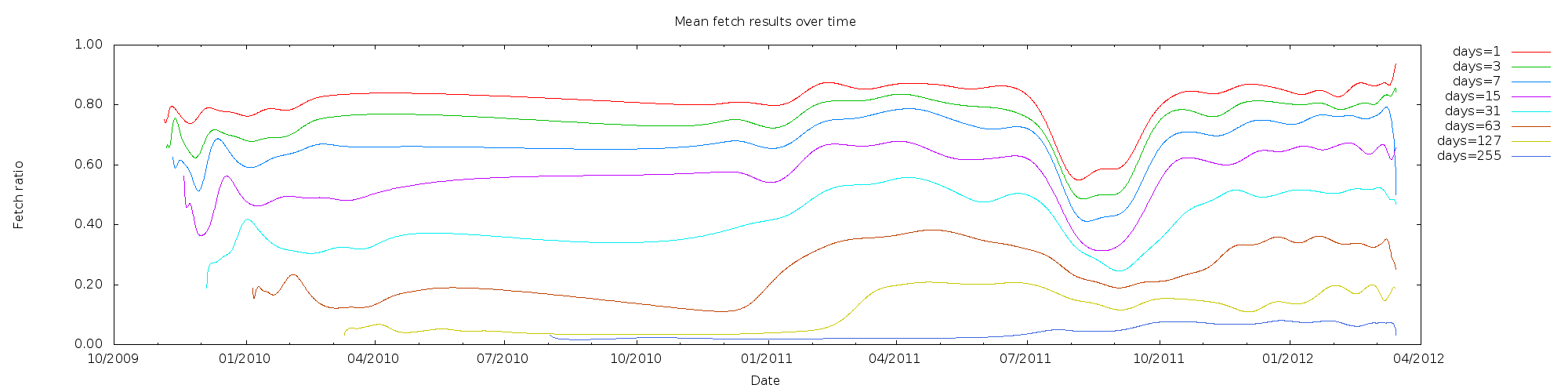
66% would be reached in the current network after about 20 days (between 2 weeks and 4 weeks), and in a zero redundancy network after 40 days. fetch-pull-stats
At the same time, though, the chunk replacement rate increased by 50%, so the mean chunk lifetime decreased by factor 2/3. So the lifetime of a file would be 4 weeks.
3.4 Generalize this
So, now we have calculations for redundancy 1, 1.5, 2 and 3. Let’s see if we can find a general (if approximate) rule for redundancy.
From the fetch-pull-graph from digger3 we see empirically, that between one week and 18 weeks each doubling of the lifetime corresponds to a reduction of the chunk retrieval probability of 15% to 20%.
Also we know that 50% probability corresponds to 4 weeks lifetime.
And we know that redundancy x has a minimum required chunk probability of 1/x.
With this, we can model the required chunk lifetime as a function of redundancy:
chunk lifetime = 4 * 2**((0.5-1/x)/0.2)
with x as redundancy. Note: this function is purely empirical and approximate.
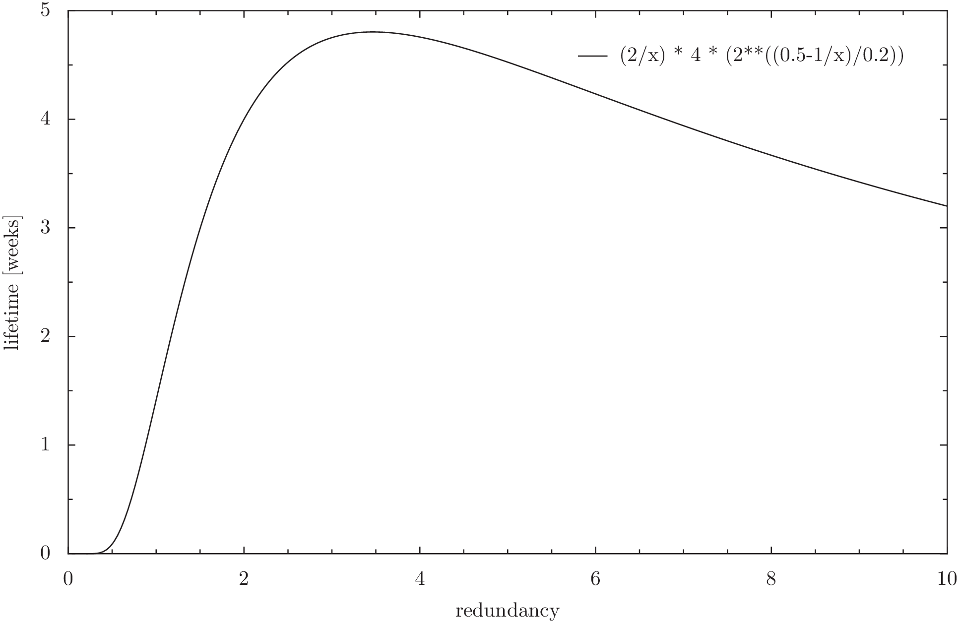
Having the chunk lifetime, we can now model the lifetime of a file as a function of its redundancy:
file lifetime = (2/x) * 4 * (2**((0.5-1/x)/0.2))
We can now use this function to find an optimum of the redundancy if we are only concerned about file lifetime. Naturally we could get the trusty wxmaxima and get the derivative of it to find the maximum. But that is not installed right now, and my skills in getting the derivatives by hand are a bit rusty (note: install running). So we just do it graphically. The function is not perfectly exact anyway, so the errors introduced by the graphic solution should not be too big compared to the errors in the model.
Note however, that this model is only valid in the range between 20% and 90% chunk retrieval probability, because the approximation for the chunk lifetime does not hold anymore for values above that. Due to this, redundancy values close to or below 1 won’t be correct.
Also keep in mind that it does not include the effect due to the higher rate of removing dead space - which is space that belongs to files which cannot be recovered anymore. This should mitigate the higher storage requirement of higher redundancy.
# encoding: utf-8
plotcmd = """
set term png
set width 15
set xlabel "redundancy"
set ylabel "lifetime [weeks]"
set output "freenet-prob-function.png"
set xrange [0:10]
plot (2/x) * 4 * (2**((0.5-1/x)/0.2))
"""
with open("plot.pyx", "w") as f:...

from subprocess import Popen
Popen(["pyxplot", "plot.pyx"])
4 Summary: Merit and outlook
Now, what do we make of this?
Firstoff: If the equations are correct, an increase in redundancy would improve the lifetime of files by a maximum of almost a week. Going further reduces the lifetime, because the increased replacement of old data outpaces the improvement due to the higher redundancy.
Also higher redundancy needs a higher storage capacity, which reduces the overall capacity of freenet. This should be partially offset by the faster purging of dead storage space.
The results support an increase in redundancy from 2 to 3, but not to 4.
Well, and aren’t statistics great? :)
Additional notes: This exploration ignores:
- healing creates less insert traffic than new inserts by only inserting failed segments, and it makes files which get accessed regularly live much longer,
- inter-segment redundancy improves the retrieving of files, so they can cope with a retrievability of 50% of any chunks of the file, even if the distribution might be skewed for a single segment,
- Non-uniformity of the network which makes it hard to model effects with global-style math like this,
- Seperate stores for SSK and CHK keys, which improve the availability of small websites and
- Usability and security impact of increased insert times (might be reduced by only inserting 2/3rd of the file data and letting healing do the rest when the first downloader gets the file)
Due to that, the findings can only provides clues for improvements, but cannot perfectly predict the best path of action. Thanks to evanb for pointing them out!
If you are interested in other applications of the same theory, you might enjoy my text Statistical constraints for the design of roleplaying games (RPGs) and campaigns (german original: Statistische Zwänge beim Rollenspiel- und Kampagnendesign). The script spielfaehig.py I used for the calculations was written for a forum discussion which evolved into that text :)
This text was written and checked in emacs org-mode and exported to HTML via `org-export-as-html-to-buffer`. The process integrated research and documentation. In hindsight, that was a pretty awesome experience, especially the inline script evaluation. I also attached the org-mode file for your leisure :)
| Anhang | Größe |
|---|---|
| freenet-prob-redundancy-2.png | 67.05 KB |
| freenet-prob-redundancy-3.png | 65.67 KB |
| freenet-prob-redundancy-4.png | 63.43 KB |
| freenet-success-probability.org | 14.84 KB |
| freenet-prob-function.png | 20.5 KB |
| fetch_dates_graph-2012-03-16.png | 17.25 KB |
| spielfaehig.py.txt | 1.15 KB |
- Druckversion
- Login to post comments
Use Node:
⚙ Babcom is trying to load the comments ⚙
This textbox will disappear when the comments have been loaded.
If the box below shows an error-page, you need to install Freenet with the Sone-Plugin or set the node-path to your freenet node and click the Reload Comments button (or return).
If you see something like Invalid key: java.net.MalformedURLException: There is no @ in that URI! (Sone/search.html), you need to setup Sone and the Web of Trust
If you had Javascript enabled, you would see comments for this page instead of the Sone page of the sites author.
Note: To make a comment which isn’t a reply visible to others here, include a link to this site somewhere in the text of your comment. It will then show up here. To ensure that I get notified of your comment, also include my Sone-ID.
Link to this site and my Sone ID: sone://6~ZDYdvAgMoUfG6M5Kwi7SQqyS-gTcyFeaNN1Pf3FvY
This spam-resistant comment-field is made with babcom.
Diese Seite nutzt Cookies. Und Bilder. Manchmal auch Text. Eins davon muss ich wohl erwähnen — sagen die meisten anderen, und ich habe grade keine Zeit, Rechtstexte dazu zu lesen…