Surface Area of regions on an ellipsoid Earth
Calculating the area of arbitrary regions on the Earth approximated as an ellipsoid. I needed this for conversion between the output of different models.
It’s calculated in Emacs Lisp, which showed me that for somewhat complex mathematical tasks Lisp syntax isn’t only unproblematic, but actually helps avoiding mistakes. And full unicode support is great for implementing algorithms with ω, λ and φ.
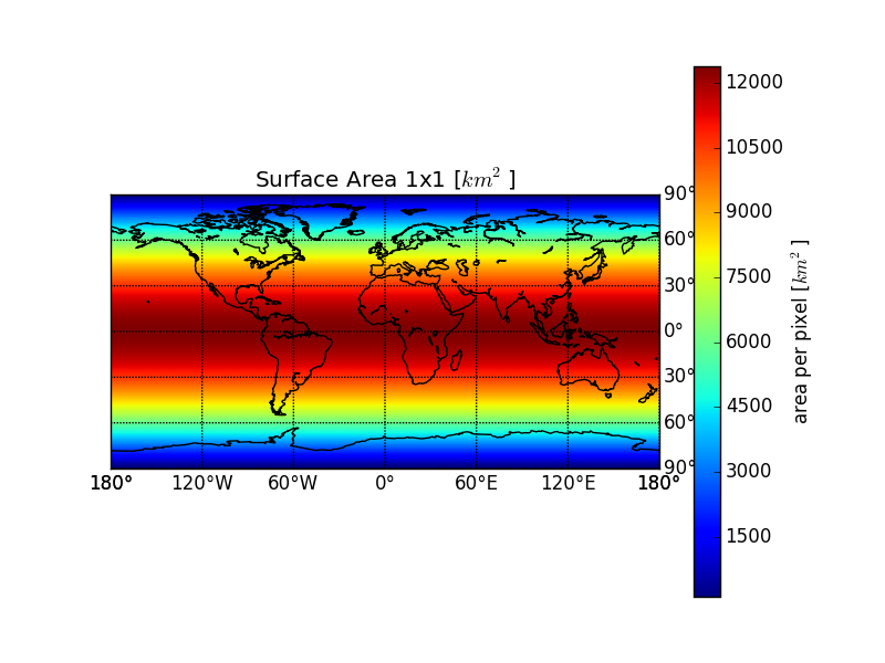
Table of Contents
1 Intro
For converting between fluxes and emissions I need the area of arbitrary regions made up of longitude×latitude pixels - specifically the transcom regions.
But the earth is no exact sphere, but rather an oblate spheroid. I need to estimate how exact I have to calculate to keep the representation errors of the regions insignificant compared to the uncertainties of the fluxes I work with.
2 Theory
http://de.wikipedia.org/wiki/Erdfigur http://de.wikipedia.org/wiki/Erdellipsoid
„Dadurch nimmt der Meeresspiegel genähert die Form eines Rotationsellipsoids an, dessen Halbachsen (Radien) sich um 21,38 km unterscheiden (a = 6378,139 ± 0,003 km ⁽¹⁾, bzw. b = 6356,752 km)“
\begin{equation} f = \frac{a-b}{a} = 1:298.25642 \pm 0.00001 \end{equation}2.1 Estimating Errors due to spherical approximation
To estimate the errors, just calculate the area of a few samples with different latitude and compare them.
Latitudes
- lat 0°
- lat 10°
- lat 30°
- lat 60°
- lat 85°
Area-Sidelength:
- 0.1°
- 1°
- 4°
2.1.1 Spherical
The simplest case for the latitude-longitude rectangle with latitude theta, longitude phi and earth radius \( R \) looks in linear approximation like this:
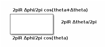
Using a cylindrical equal area rectangle projection (Lambert) we can calculate the area of a given latitude-longitude square as follows:
With θ as longitude, φ as latitude and \( R \) as radius of the earth sphere.
For a 1°×1° square, that equals
(defun spherecutarea (latdeg sidelength deglen)
  "Calculate the area of a cut in a sphere at the latitude LATDEG
with the given SIDELENGTH and the length of one degree at the
Equator DEGLEN."
  (* deglen sidelength ; longitude
     deglen sidelength (cos (* 2 float-pi (/ latdeg 360.0))))) ; latitude

(defun spherearea (latdeg sidelength)
  "Area of a segment of a sphere at LATDEG with the given
SIDELENGTH."
  (let* ((R 6371.0) ; km
         (deglen (/ (* 2 float-pi R) 360.0))) ; km^2
    (spherecutarea latdeg sidelength deglen)))
| latitude ↓ | 0.1 | 1 | 4 |
|---|---|---|---|
| 0 | 123.64 | 12364.31 | 197828.99 |
| 10 | 121.76 | 12176.47 | 194823.52 |
| 30 | 107.08 | 10707.81 | 171324.93 |
| 60 | 61.82 | 6182.16 | 98914.49 |
| 85 | 10.78 | 1077.62 | 17241.93 |
(defun spheresegmentarea (latdeg sidelength)
  "Calculate the area of a rectangular segment on a sphere at
latitude LATDEG with the given SIDELENGTH."
  (* 24728.6234228 sidelength sidelength
     (cos (* float-pi (/ latdeg 180.0)))))
spheresegmentarea
2.2 Simple ellipsoid integral (scrapped)
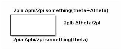
Instead of the very simple spherical compression, we can use integration over the area of an oblated spheroid, or more exactly: an ellipsoid of revolution.
An oblated spheroid has one short axis and two long axi. For the earth, the short axis is the polar radius \( b = 6356,752 km \) while the long axi have the length of the equatorial radius \( a = a = 6378,139 ± 0,003 km \).
Thus the linear approximation of an area on the spheroid looks like this:
Let’s scrap that. I’m drowning in not-so-simple ideas, so I’d rather take a pre-generated formula, even if it means cutting leafs with a chainsaw. Let’s go to an astronomy book: Astronomische Algorithmen by Jean Meeus has a formula for distances on an ellipsoid.
2.3 Square approximation with ellipsoid sidelength calculation
Taking the algorithm from Astronomische Algorithmen rev. 2 by Jean Meeus. I want to know how big the errors are when I just take a circle. So let’s implement a fitting algorithm.
The following algorithm gives us the distance between two points.
\begin{equation} F = \frac{\phi_1 + \phi_2}{2}, G = \frac{\phi_1 - \phi_2}{2}, \lambda = \frac{L_1 - L_2}{2} \end{equation} \begin{equation} S = sin^2 G ~ cos^2 G + cos^2 F ~ sin^2 \lambda \end{equation} \begin{equation} C = cos^2 G ~ cos^2 G + sin^2 F ~ sin^2 \lambda \end{equation} \begin{equation} tan \omega = \sqrt{\frac{S}{C}} \end{equation} \begin{equation} R = \frac{\sqrt{SC}}{\omega} , ~ omega ~ in ~ radians \end{equation} \begin{equation} D = 2 \omega a \end{equation} \begin{equation} H_1 = \frac{3R - 1}{2C}, H_2 = \frac{3R + 2}{2S} \end{equation} \begin{equation} s = D(1 + fH_1 ~ sin^2 F ~ cos^2 G - fH_2 ~ cos^2 F ~ sin^2 G) \end{equation}We can now use the distance \( s \) between the 4 corners of a pseudo-rectangular area on the ellipsoid to approximate the area of the pseudo-square they delimit.
\begin{equation} A = \frac{s_{bottomright - bottomleft} + s_{topright - topleft}}{2} \cdot s_{topleft - bottomleft} \end{equation}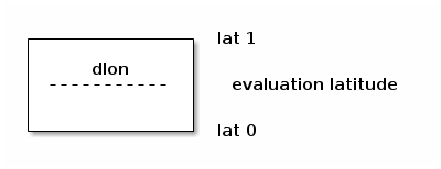
But by doing so we treat the non-linear problem as linear. To minimize the error, we can split an area into many smaller areas and sum up their areas (numerical approximation).
In following we will use the direct algorithm as well as the numerical approximation.
2.3.1 Code
(defmacro turntofloatsingle (var)
  (list 'setq var (list 'float var)))

(defmacro turntofloat (&rest vars)
  "Turn a list of items to floats."
  (cons 'progn (mapcar
                (lambda (var)
                  (list 'turntofloatsingle var))
                vars)))
(defun ellipsoiddistance (a f L1 L2 φ1 φ2)
  "Calculate the distance of two arbitrary points on an ellipsoid.

  Parameters: Equator radius A, oblateness F and for point 1 and
  2 respectively the longitudes L1 and L2 and the latitudes φ1
  and φ2."
  ; ensure that we work on floats
  (turntofloat a f φ1 φ2 L1 L2)
  ; the first simplifications don’t depend on each other,
  ; so we just use let to bind them
  (let ((F (/ (+ φ1 φ2) 2))
        (G (/ (- φ1 φ2) 2))
        (λ (/ (- L1 L2) 2)))
    (message (format "F %f G %f λ %f a %f f %f L1 %f L2 %f φ1 %f φ2 %f"
                     F G λ a f L1 L2 φ1 φ2))
    ; the second don’t depend on each other either
    (let ((S (+ (* (expt (sin G) 2)
                   (expt (cos λ) 2))
                (* (expt (cos F) 2)
                   (expt (sin λ) 2))))
          (C (+ (* (expt (cos G) 2)
                   (expt (cos λ) 2))
                (* (expt (sin F) 2)
                   (expt (sin λ) 2)))))
      ; now we have a few consecutive definitions, so we use let*
      ; which allows references to previous elements in the same let*.
      (let* ((ω (atan (sqrt (/ S C))))
             (R (/    (sqrt (* S C)) ω)))
        (let ((D (* 2 ω a))
              (H1 (/ (- (* 3 R)) (* 2 C)))
              (H2 (/ (+ (* 3 R)) (* 2 C))))
          ; All prepared. Now we just fit all this together. This is
          ; the last line, so the function returns the value.
          (* D (-
                (+ 1 (* f H1 (expt (sin F) 2) (expt (cos G) 2)))
                (* f H2 (expt (cos F) 2) (expt (sin G) 2)))))))))
(defun ellipsoidrectanglearea (a f longitude latitude dlon dlat)
  (let ((L1 longitude)
        (L2 (+ longitude dlon))
        (φ1 latitude)
        (φ2 (+ latitude dlat)))
    (let ((lenlower (ellipsoiddistance a f L1 L2 φ1 φ1))
          (lenupper (ellipsoiddistance a f L1 L2 φ2 φ2))
          (lenwestern (ellipsoiddistance a f L1 L1 φ1 φ2))
          (leneastern (ellipsoiddistance a f L2 L2 φ1 φ2)))
      (if (not (= lenwestern leneastern))
          (error "Western and Eastern length are not equal.
This violates the laws of geometry. We die. Western: %f Eastern: %f"
                 lenwestern leneastern))
      (let ((horizontalmean (/ (+ lenlower lenupper) 2)))
        ; now just return length times width
        (* horizontalmean lenwestern)))))
<<ellipsoid-helpers>>
<<ellipsoid-distance>>
<<ellipsoid-rectanglearea>>

(defun ellipsoidrectangleareafromdeg (latdeg sidelength)
  "Calculate the rectangle area from the latitude LATDEG and the
SIDELENGTH given as degrees."
  (message (format "latdeg %f sidelength %f" latdeg sidelength))
  (let ((londeg 15) ; irrelevant due to symmetry
        (dlondeg sidelength)
        (dlatdeg sidelength)
        (a 6378.139)
        (f (/ 1 298.25642)))
    (let ((lon (* 2 float-pi (/ londeg 360.0))) ; 2π / 360
          (dlon (* 2 float-pi (/ dlondeg 360.0)))
          (lat (* 2 float-pi (/ latdeg 360.0)))
          (dlat (* 2 float-pi (/ dlatdeg 360.0))))
      (ellipsoidrectanglearea a f lon lat dlon dlat))))

(defun ellipsoidrectangleareafromdegnumericalintegration (latdeg sidelength steps)
  "Calculate the rectangle area from the latidute LATDEG and the
  SIDELENGTH given as degrees by adding them in STEPS smaller steps per sidelength."
  (let ((area 0)
        (smallerside (/ (float sidelength)
                        (float steps))))
    (loop for i from 0 to (1- steps) by 1 do
          (message (format "i %f" i))
          (let ((smallerlat (+ latdeg (* smallerside i))))
            ; add stepts times the area since the longitudinal
            ; calculation does not change, so we only need to
            ; calculate in once.
            (setq area (+ area (* steps
                                  (ellipsoidrectangleareafromdeg
                                   smallerlat smallerside))))))

    area))
; no return value
nil
2.3.2 Results for direct calculation
| latitude ↓ | 0.1 | 1 | 4 |
|---|---|---|---|
| 0 | 123.9203 | 12391.0741 | 198026.1548 |
| 10 | 121.9815 | 12179.9838 | 193733.6082 |
| 20 | 116.2724 | 11592.4962 | 183457.2705 |
| 30 | 106.9937 | 10649.2503 | 167557.9088 |
| 40 | 94.4643 | 9382.6379 | 146580.1726 |
| 45 | 87.1079 | 8640.9234 | 134399.3469 |
| 50 | 79.1019 | 7834.8158 | 121219.4843 |
| 60 | 61.4002 | 6055.4408 | 92285.3707 |
| 70 | 41.9067 | 4099.4608 | 60666.5036 |
| 80 | 21.2036 | 2025.2137 | 27301.2374 |
| 85 | 10.5861 | 962.5255 | 10264.8590 |
| 90 | 0.1071 | 107.0494 | 6844.8700 |
2.3.3 Results for summing up smaller squares.
- 100 squares per area (10 latitude steps)
Table 3: Area of lat-lon “square” with the given sidelength in \(km^2\) sum 10 latitude ↓ 0.1 1 4 0 123.9203 12391.3918 198107.5151 10 121.9815 12180.3007 193814.7025 20 116.2724 11592.8099 183537.3359 30 106.9937 10649.5549 167635.3476 40 94.4643 9382.9239 146652.3820 45 87.1079 8641.1954 134467.6868 50 79.1019 7835.0702 121283.0172 60 61.4002 6055.6486 92336.3892 70 41.9067 4099.6076 60701.4093 80 21.2036 2025.2881 27317.3197 85 10.5862 962.5611 10270.9364 90 0.1071 107.0533 6848.9244 - 10000 squares per area (100 latitude steps)
Table 4: Area of lat-lon “square” with the given sidelength in \(km^2\) sum 100 latitude ↓ 0.1 1 4 0 123.9203 12391.3950 198108.3283 10 121.9815 12180.3039 193815.5131 20 116.2724 11592.8130 183538.1364 30 106.9937 10649.5580 167636.1220 40 94.4643 9382.9268 146653.1043 45 87.1079 8641.1981 134468.3705 50 79.1019 7835.0727 121283.6529 60 61.4002 6055.6507 92336.8997 70 41.9067 4099.6090 60701.7587 80 21.2036 2025.2888 27317.4807 85 10.5862 962.5615 10270.9973 90 0.1071 107.0534 6848.9650 - 1000000 squares per area (1000 latitude steps)
Table 5: Area of lat-lon “square” with the given sidelength in \(km^2\) sum 1000 latitude ↓ 0.1 1 4 0 123.9203 12391.3950 198108.3365 10 121.9815 12180.3039 193815.5213 20 116.2724 11592.8130 183538.1444 30 106.9937 10649.5580 167636.1297 40 94.4643 9382.9268 146653.1115 45 87.1079 8641.1982 134468.3773 50 79.1019 7835.0728 121283.6592 60 61.4002 6055.6507 92336.9048 70 41.9067 4099.6090 60701.7621 80 21.2036 2025.2888 27317.4823 85 10.5862 962.5615 10270.9979 90 0.1071 107.0534 6848.9654 - 10 steps vs 1 step, relative
Table 6: Area of lat-lon “square” with the given sidelength in \(km^2\) 10 vs. 1 latitude ↓ 0.1 1 4 0 0.0000% 0.0026% 0.0411% 10 0.0000% 0.0026% 0.0419% 20 0.0000% 0.0027% 0.0436% 30 0.0000% 0.0029% 0.0462% 40 0.0000% 0.0030% 0.0493% 45 0.0000% 0.0031% 0.0508% 50 0.0000% 0.0032% 0.0524% 60 0.0000% 0.0034% 0.0553% 70 0.0000% 0.0036% 0.0575% 80 0.0000% 0.0037% 0.0589% 85 0.0000% 0.0037% 0.0592% 90 0.0000% 0.0037% 0.0592% - 100 steps vs 10 steps, relative
Table 7: Area of lat-lon “square” with the given sidelength in \(km^2\) 100 vs. 10 latitude ↓ 0.1 1 4 0 0.000000% 0.000026% 0.000410% 10 0.000000% 0.000026% 0.000418% 20 0.000000% 0.000027% 0.000436% 30 0.000000% 0.000029% 0.000462% 40 0.000000% 0.000030% 0.000493% 45 0.000000% 0.000031% 0.000508% 50 0.000000% 0.000032% 0.000524% 60 0.000000% 0.000034% 0.000553% 70 0.000000% 0.000036% 0.000576% 80 0.000000% 0.000037% 0.000589% 85 0.000000% 0.000037% 0.000592% 90 0.000000% 0.000037% 0.000593% - 1000 steps vs 100 steps, relative
Table 8: Area of lat-lon “square” with the given sidelength in \(km^2\) 1000 vs 100 latitude ↓ 0.1 1 4 0 0.000000% 0.000000% 0.000004% 10 0.000000% 0.000000% 0.000004% 20 0.000000% 0.000000% 0.000004% 30 0.000000% 0.000000% 0.000005% 40 0.000000% 0.000000% 0.000005% 45 0.000000% 0.000000% 0.000005% 50 0.000000% 0.000000% 0.000005% 60 0.000000% 0.000000% 0.000006% 70 0.000000% 0.000000% 0.000006% 80 0.000000% 0.000000% 0.000006% 85 0.000000% 0.000000% 0.000006% 90 0.000000% 0.000000% 0.000006%
3 Implementation
This is almost done in the theory. Only thing left to do: Use the algorithm to generate a list of areas per 1° latitude and pass that to a python script which writes it into a netCDF4 file for later usage.
I need a python snippet which takes a list of values from lat 0° to lat 90° as input and turns it into a 360°×180° map.
Or I could just write the data from the elisp code to a file and read that.
3.1 Write data files
<<ellipsoidrectangleareafromdeg>>
(with-temp-file "transcomellipticlat90-sum1000.dat"
  ; switch to the opened file
  (switch-to-buffer (current-buffer))
  (loop for lat from 0 to 90 do
        (insert (concat (number-to-string lat) " "))
        (insert (number-to-string
                 (ellipsoidrectangleareafromdegnumericalintegration lat 1 1000)))
        (insert "\n")))
; dang, this is beautiful!
<<ellipsoidrectangleareafromdeg>>
(with-temp-file "transcomellipticlat90-direct.dat"
  ; switch to the opened file
  (switch-to-buffer (current-buffer))
  (loop for lat from 0 to 90 do
        (insert (concat (number-to-string lat) " "))
        (insert (number-to-string
                 (ellipsoidrectangleareafromdegnumericalintegration lat 1 1)))
        (insert "\n")))
<<ellipsoidrectangleareafromdeg>>
(with-temp-file "transcomellipticlat90-sum1000vsdirect.dat"
  ; switch to the opened file
  (switch-to-buffer (current-buffer))
  (loop for lat from 0 to 90 do
        (insert (concat (number-to-string lat) " "))
        (insert (number-to-string
                 (- (ellipsoidrectangleareafromdegnumericalintegration lat 1 1000)
                    (ellipsoidrectangleareafromdegnumericalintegration lat 1 1))))
        (insert "\n")))
<<ellipsoidrectangleareafromdeg>>
<<spherearea>>
(with-temp-file "transcomellipticlat90-sum1000vssphere.dat"
  ; switch to the opened file
  (switch-to-buffer (current-buffer))
  (loop for lat from 0 to 90 do
        (insert (concat (number-to-string lat) " "))
        (insert (number-to-string
                 (- (ellipsoidrectangleareafromdegnumericalintegration lat 1 1000)
                    (spherearea lat 1))))
        (insert "\n")))
<<spherearea>>
(with-temp-file "transcomellipticlat90-sphere.dat"
  ; switch to the opened file
  (switch-to-buffer (current-buffer))
  (loop for lat from 0 to 90 do
        (insert (concat (number-to-string lat) " "))
        (insert (number-to-string (spherearea lat 1)))
        (insert "\n")))
(with-temp-file "transcomellipticlat90-sum1000vssphere.dat"
  ; switch to the opened file
  (switch-to-buffer (current-buffer))
  (loop for lat from 0 to 90 do
        (insert (concat (number-to-string lat) " "))
        (insert (number-to-string (- (ellipsoidrectangleareafromdegnumericalintegration lat 1 1000) (spheresegmentarea lat 1))))
        (insert "\n")))
3.2 Write datafiles to netcdf and plot them
Now just readout that file as csv
3.2.1 First define the plotstyle
The following codeblock can be summoned into other code via
<<addplotstyle>>
# add map lines
m.drawcoastlines()
m.drawparallels(np.arange(-90.,120.,30.),
                labels=[False,True,True,False])
m.drawmeridians(np.arange(0.,420.,60.),
                labels=[True,False,False,True])
m.drawmapboundary(fill_color='aqua')
3.2.2 Now read datafiles
import numpy as np
import pylab as pl
import mpl_toolkits.basemap as bm
import netCDF4 as nc
def singlehemispherelats2map(northernlats):
    """Turn the northern lats (0-90) into a map (180,360)."""
    # duplicate the northernlats
    lats = np.zeros((180, ))
    lats[0:90] = northernlats[:0:-1,1]
    lats[90:] = northernlats[1:,1]
    # and blow them up into a map
    lons = np.ones((360, ))
    lats = np.matrix(lats)
    lons = np.matrix(lons)
    mapscaling = lons.transpose() * lats
    mapscaling = mapscaling.transpose()
    return mapscaling

# first read the file
with open("transcomellipticlat90-sum1000.dat") as f:
    northernlats = np.genfromtxt(f, delimiter=" ")
mapscaling = singlehemispherelats2map(northernlats)
with open("transcomellipticlat90-sum1000vsdirect.dat") as f:
    northernlats = np.genfromtxt(f, delimiter=" ")
mapscalingdiff = singlehemispherelats2map(northernlats)
with open("transcomellipticlat90-direct.dat") as f:
    northernlats = np.genfromtxt(f, delimiter=" ")
mapscalingdirect = singlehemispherelats2map(northernlats)
with open("transcomellipticlat90-sphere.dat") as f:
    northernlats = np.genfromtxt(f, delimiter=" ")
mapscalingsphere = singlehemispherelats2map(northernlats)
with open("transcomellipticlat90-sum1000vssphere.dat") as f:
    northernlats = np.genfromtxt(f, delimiter=" ")
mapscalingdiffsphere = singlehemispherelats2map(northernlats)
3.2.3 and plot them
# several different plots:
<<plotareamapperpixel>>
<<plotareamapperpixeldirect>>
<<plotareamapperpixelerror>>
<<plotareamapperpixelrelerror>>
<<plotareamapperpixelsphereerror>>
# plot it for representation
m = bm.Basemap()
m.imshow(mapscaling)
bar = pl.colorbar()
bar.set_label("area per pixel [$km^2$]")
<<addplotstyle>>
pl.title("Surface Area 1x1 [$km^2$]")
pl.savefig("eartharea_1x1.png")
pl.close()
print """\n\n#+caption:Area when summing 1000x1000 smaller areas
[[./eartharea_1x1.png]]"""
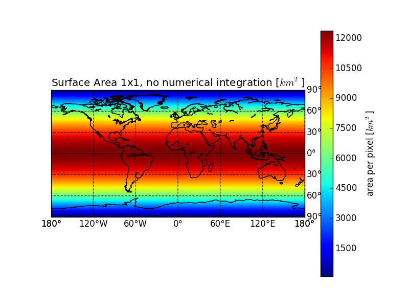
m = bm.Basemap()
m.imshow(mapscaling)
bar = pl.colorbar()
bar.set_label("area per pixel [$km^2$]")
# summon map style! :)
<<addplotstyle>>
pl.title("Surface Area 1x1, no numerical integration [$km^2$]")
pl.savefig("earthareadirect_1x1.png")
pl.close()
print "\n\n#+caption:Area when using just one square\n[[./earthareadirect_1x1.png]]"
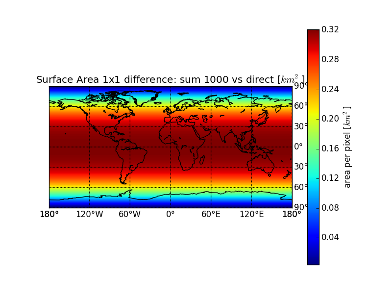
m = bm.Basemap()
m.imshow(mapscalingdiff)
<<addplotstyle>>
bar = pl.colorbar()
bar.set_label("area per pixel [$km^2$]")
pl.title("Surface Area 1x1 difference: sum 1000 vs direct [$km^2$]")
pl.savefig("eartharea1000vs1_1x1.png")  # save as a clean netCDF4 file
pl.close()
print "\n\n#+caption:Difference between summing smaller squares",
print "and just using one square\n[[./eartharea1000vs1_1x1.png]]"
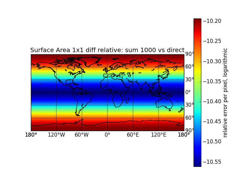
m = bm.Basemap()
m.imshow(np.log(np.abs(mapscalingdiff/mapscaling)))
<<addplotstyle>>
bar = pl.colorbar()
bar.set_label("relative error per pixel, logarithmic")
pl.title("Surface Area 1x1 diff relative: sum 1000 vs direct")
pl.savefig("eartharea1000vs1rel_1x1.png")  # save as a clean netCDF4 file
pl.close()
print """\n\n#+caption:Relative Area Error by not integrating (logscale)
[[./eartharea1000vs1rel_1x1.png]]"""
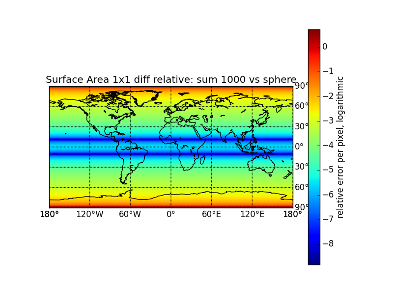
m = bm.Basemap()
m.imshow(np.log(np.abs(mapscalingdiffsphere/mapscaling)))
<<addplotstyle>>
bar = pl.colorbar()
bar.set_label("relative error per pixel, logarithmic")
pl.title("Surface Area 1x1 diff relative: sum 1000 vs sphere")
pl.savefig("eartharea1000vssphererel_1x1.png")
pl.close()
print """\n\n#+caption:Relative Error from Sphere (logscale)
[[./eartharea1000vssphererel_1x1.png]]"""
3.2.4 Write the data
<<readcsvareafiles>>
<<plotareamaps>>
D = nc.Dataset("eartharea.nc", "w")
D.comment = "Created with tm5tools/ct2pyshell/transcomareas.org"
D.createDimension("longitude", 360)
D.createDimension("latitude", 180)
area = D.createVariable("1x1", "f8", ("latitude", "longitude"))
area.units = "km^2"
area.comment = "from 180W to 180E and from 90S to 90N"
area[:] = mapscaling
area = D.createVariable("1x1_1000vs1", "f8", ("latitude", "longitude"))
area.units = "km^2"
area.comment = ("Difference between the direct calculation of the "
"area and summing up 1000x1000 smaller areas."
"from 180W to 180E and from 90S to 90N")
area[:] = mapscalingdiff
area = D.createVariable("1x1_direct", "f8", ("latitude", "longitude"))
area.units = "km^2"
area.comment = ("Area calculated without numerical intergration (bigger errors!). "
"from 180W to 180E and from 90S to 90N")
area[:] = mapscalingdirect
area = D.createVariable("1x1_sphere", "f8", ("latitude", "longitude"))
area.units = "km^2"
area.comment = ("Area calculated on a simple sphere. "
"from 180W to 180E and from 90S to 90N")
area[:] = mapscalingsphere
4 Validation
4.1 Surface Area of the Earth
Should be around 510 million km²
(let ((s 0))
  (loop for lat from 0 to 90 do
        (setq s (+ s (spherearea lat 1))))
  (/ (* 2 360 s) 1.0e6)) ; million kilometers
514.5026761832414
(let ((s 0))
  (loop for lat from 0 to 90 do
        (setq s (+ s (ellipsoidrectangleareafromdegnumericalintegration lat 1 1))))
  (/ (* 2 360 s) 1.0e6)) ; million kilometers
509.55872913305257
(let ((s 0))
  (loop for lat from 0 to 90 do
        (setq s (+ s (ellipsoidrectangleareafromdegnumericalintegration lat 1 10))))
  (/ (* 2 360 s) 1.0e6)) ; million kilometers
509.57373786401286
(let ((s 0))
  (loop for lat from 0 to 90 do
        (setq s (+ s (ellipsoidrectangleareafromdegnumericalintegration lat 1 1000))))
  (/ (* 2 360 s) 1.0e6)) ; million kilometers
509.5738894527161
4.2 Area of Australia + New Zealand (Transcom Region 10)
Should be around 7,692,024 km² + 269,652 km² = 7,961,676 km²
import netCDF4 as nc
import numpy as np
import pylab as pl

D = nc.Dataset("eartharea.nc")
area = D.variables["1x1"][:]
T = nc.Dataset("../plotting/transcom_regions_ct/regions.nc")
transcom = T.variables["transcom_regions"][:]
mask = transcom[::-1,:] == 10
pl.imshow(mask*area)
bar = pl.colorbar()
bar.set_label("area per pixel [$km^2$]")
pl.title("Area of Australia and New Zealand in [$km^2$] per pixel")
pl.savefig("area-australia.png")
# pl.show()
return np.sum(mask*area)
7976938.58492
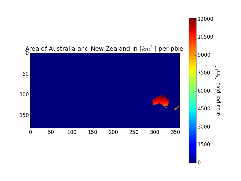
Figure 1: Area of Australia and New Zealand
5 Summary
The area of 1x1 degree pixels on a worldmap in ellipsoid approximation is available in the file eartharea.nc in the variable “1x1”. Visualized it looks like this:
Figure 2: Surface Area of the Earth in \(km^2\)
To calculate the emissions from mol/m², just multiply each gridpoint with 106 m²/km² and the gridpoint in the variable:
<<prep>>
import numpy as np
import pylab as pl
import mpl_toolkits.basemap as bm
import netCDF4 as nc
D = nc.Dataset("eartharea.nc")
area = D.variables["1x1"][:]
flux = np.ones((180, 360)) * np.random.normal(0.0, 1.e-6, (180, 360))
emiss = flux*area
m = bm.Basemap()
m.imshow(emiss)
<<addplotstyle>>
bar = pl.colorbar()
bar.set_label("emissions [mol/s]")
pl.title("random flux $0 \pm 1.e-6 \\frac{mol}{m^{2}s}$ turned to random emissions")
filename = "randomemissions.png"
pl.savefig(filename)
print "#+caption: Random emissions in simple lat/lon plot."
print "[[./" +  filename + "]]"
# plot again, with hobo-dyer projection (equal-area)
pl.close()
m = plotmap(emiss)
<<addplotstyle>>
bar = pl.colorbar()
bar.set_label("emissions [mol/s]")
pl.title("random emissions in hobo-dyer projection")
filename = "randomemissionshobo-dyer.png"

pl.savefig(filename)
print """\n\n#+caption: Random Emissions in Hobo Dyer Projection
[[./""" +  filename + "]]"
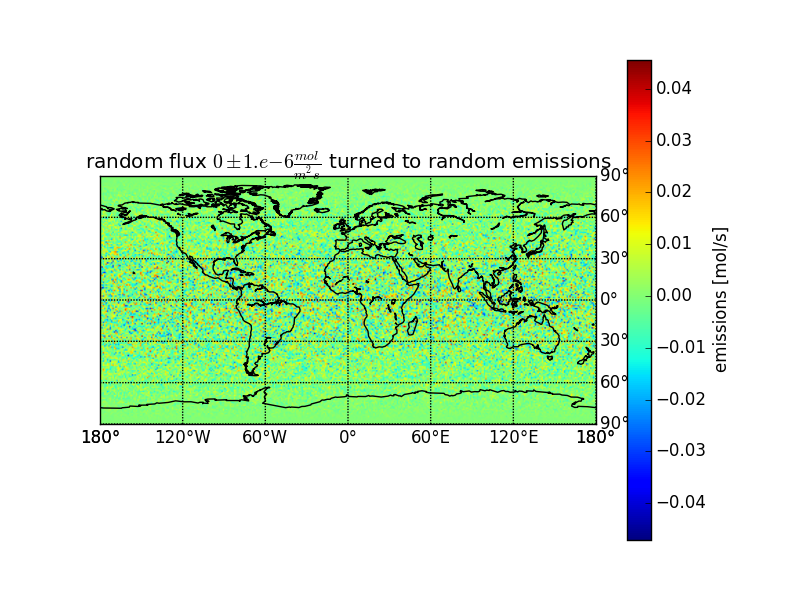
Figure 3: Random emissions in simple lat/lon plot.
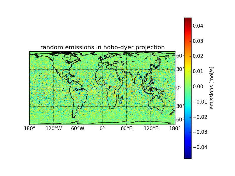
Figure 4: Random Emissions in Hobo Dyer Projection
def plotmap(array):
    """Plot an array as map."""
    m = bm.Basemap(projection='cea', lat_ts=37.5)
    ny, nx = array.shape[:2]
    lons, lats = pl.meshgrid(range(-nx/2, nx/2 + nx%2),
                             range(-ny/2, ny/2 + ny%2))
    x, y = m(lons, lats)
    arr = array.copy()
    for i in arr.shape[2:]:
        arr = arr[:,:,0]
    m.pcolormesh(x, y, arr)
    return m
5.1 Landarea
Estimating the land area for a given lat-lon region (this requires a
land/sea map in the file t3_regions_landsea.nc, i.e. from TM5-4DVar,
see tm5.sf.net).
<<prep>>
import netCDF4 as nc
import numpy as np
import pylab as pl
import mpl_toolkits.basemap as bm


def landarea(lat0, lon0, lat1, lon1):
    """Calculate the land area in the rectangle defined by the
    arguments.

    :param lat0: latitude in degree. Southern Hemisphere negative.
    :param lon0: longitude in degree. East negative.

    :returns: landarea within the rectangle in km^2

    >>> samarea = 17.840 * 1000000 # km^2
    >>> ae = landarea(15, -90, -60, -30)
    >>> 0.99 * samarea < ae < 1.01 * samarea
    True
    """
    lat0idx = int(lat0 + 90)
    lat1idx = int(lat1 + 90)
    if lat0idx > lat1idx:
        tmp = lat1idx
        lat1idx = lat0idx
        lat0idx = tmp
    lon0idx = int(lon0 + 180)
    lon1idx = int(lon1 + 180)
    if lon0idx > lon1idx:
        tmp = lon1idx
        lon1idx = lon0idx
        lon0idx = tmp
    D = nc.Dataset("eartharea.nc")
    T = nc.Dataset("t3_regions_landsea.nc")
    area = D.variables["1x1"][:]
    landfraction05x05 = T.variables["LSMASK"][:]
    landfraction1x1 = np.zeros((180,360)) # latxlon
    for i in range(landfraction1x1.shape[0]):
        for j in range(landfraction1x1.shape[1]):
            landfraction1x1[i,j] = np.mean(landfraction05x05[i*2:i*2+2,:][:,j*2:j*2+2])
    landarea = area * landfraction1x1
    # m = plotmap(landfraction1x1)
    # pl.show()
    # m = plotmap(landarea)
    # pl.show()
    return np.sum(landarea[lat0idx:lat1idx+1,:][:,lon0idx:lon1idx])


if True or __name__ == "__main__":
    import doctest
    doctest.testmod()
6 Notes
6.1 Understanding the macro to turn variables to float
Most of the code snippets here are thanks to ggole in #emacs on irc.freenode.net (What is IRC?).
6.1.1 Single variable
(defmacro turntofloatsingle (var)
  (list 'setq var (list 'float var)))
6.1.2 Backtick notation
<<turntofloat-single>>
(defmacro turntofloatbackticks (&rest vars)
  "Turn a list of items to floats using backtick notation."
  `(progn ,@(mapcar
             (lambda (var)
               `(turntofloatsingle ,var))
             vars)))
6.1.3 Use Mapcar
<<turntofloat-single>>
(defmacro turntofloat (&rest vars)
  "Turn a list of items to floats (without using backticks)."
  ; cons turns this into a call of progn on the list returned by
  ; mapcar
  (cons 'progn (mapcar
                (lambda (var)
                  (list 'turntofloatsingle var))
                vars)))
6.1.4 Common Lisp collect
<<turntofloat-single>>
(defmacro turntofloatcollect (&rest vars)
  "Turn a list of items to floats, using the collect directive of loop."
  ; execute progn on the list returned by the loop
  (cons 'progn
        ; loop ... collect returns a list of all the loop results.
        (loop for var in vars collect
              (list 'turntofloatsingle var))))
6.1.5 Explicit List Building
<<turntofloat-single>>

; build the list explicitely to make it easier for me to understand
; what the macro does
(defmacro turntofloatexplicit (&rest vars)
  "Turn a list of items to floats (using explicit list building
instead of mapcar)."
  ; prepare an empty list of function calls
  (let ((funclist '()))
    ; for each variable add a call to the single-item macro
    (loop for var in vars do
          ; (list 'turntofloatsingle var) creates the call to
          ; turntofloatsingle with the variable which is referenced by
          ; var. Push puts that at the beginning of the funclist.
          (push (list 'turntofloatsingle var) funclist))
    ; to ensure the right order of operations, we reverse the funclist
    (setq funclist (reverse funclist))
    ; cons turns this into a call of progn on the list. We need progn,
    ; because the funclist contains multiple function calls.
    (cons 'progn funclist)))
6.1.6 Mapcar and Callf
<<turntofloat-single>>
; Common Lisp Macro to turn the place to a float in one step.
(defmacro turntofloatinline (&rest places)
  "Turn a list of items to floats using an inline function call."
  `(progn ,@(mapcar
             (lambda (place)
               `(callf float ,place)) places)))
6.1.7 Test the results
<<turntofloat-collect>>
(setq a 1 b 3.8 c 2)
(turntofloatcollect a b c)
(message (number-to-string c))
| Anhang | Größe |
|---|---|
| eartharea-eartharea_1x1.png | 88.19 KB |
| eartharea.nc | 1.98 MB |
| eartharea.pdf | 1.19 MB |
| eartharea-area-australia.png | 33.3 KB |
| eartharea-eartharea1000vs1_1x1.png | 86.35 KB |
| eartharea-eartharea1000vssphererel_1x1.png | 98.72 KB |
| eartharea-eartharea1000vs1rel_1x1.png | 92.39 KB |
| eartharea-eartharea_1x1.png | 88.19 KB |
| eartharea-earthareadirect_1x1.png | 90.13 KB |
| eartharea-randomemissions.png | 353.01 KB |
| eartharea-randomemissionshobo-dyer.png | 239.52 KB |
| eartharea-segmentellipsoid.png | 5.39 KB |
| eartharea-segmentellipsoiddistances.png | 2.72 KB |
| eartharea-segmentsphere.png | 5.24 KB |
| eartharea.org | 42.75 KB |
- Druckversion
- Login to post comments
Use Node:
⚙ Babcom is trying to load the comments ⚙
This textbox will disappear when the comments have been loaded.
If the box below shows an error-page, you need to install Freenet with the Sone-Plugin or set the node-path to your freenet node and click the Reload Comments button (or return).
If you see something like Invalid key: java.net.MalformedURLException: There is no @ in that URI! (Sone/search.html), you need to setup Sone and the Web of Trust
If you had Javascript enabled, you would see comments for this page instead of the Sone page of the sites author.
Note: To make a comment which isn’t a reply visible to others here, include a link to this site somewhere in the text of your comment. It will then show up here. To ensure that I get notified of your comment, also include my Sone-ID.
Link to this site and my Sone ID: sone://6~ZDYdvAgMoUfG6M5Kwi7SQqyS-gTcyFeaNN1Pf3FvY
This spam-resistant comment-field is made with babcom.
Diese Seite nutzt Cookies. Und Bilder. Manchmal auch Text. Eins davon muss ich wohl erwähnen — sagen die meisten anderen, und ich habe grade keine Zeit, Rechtstexte dazu zu lesen…